Plot TOST Equivalence-Test Power Curves Over a Range of True Differences

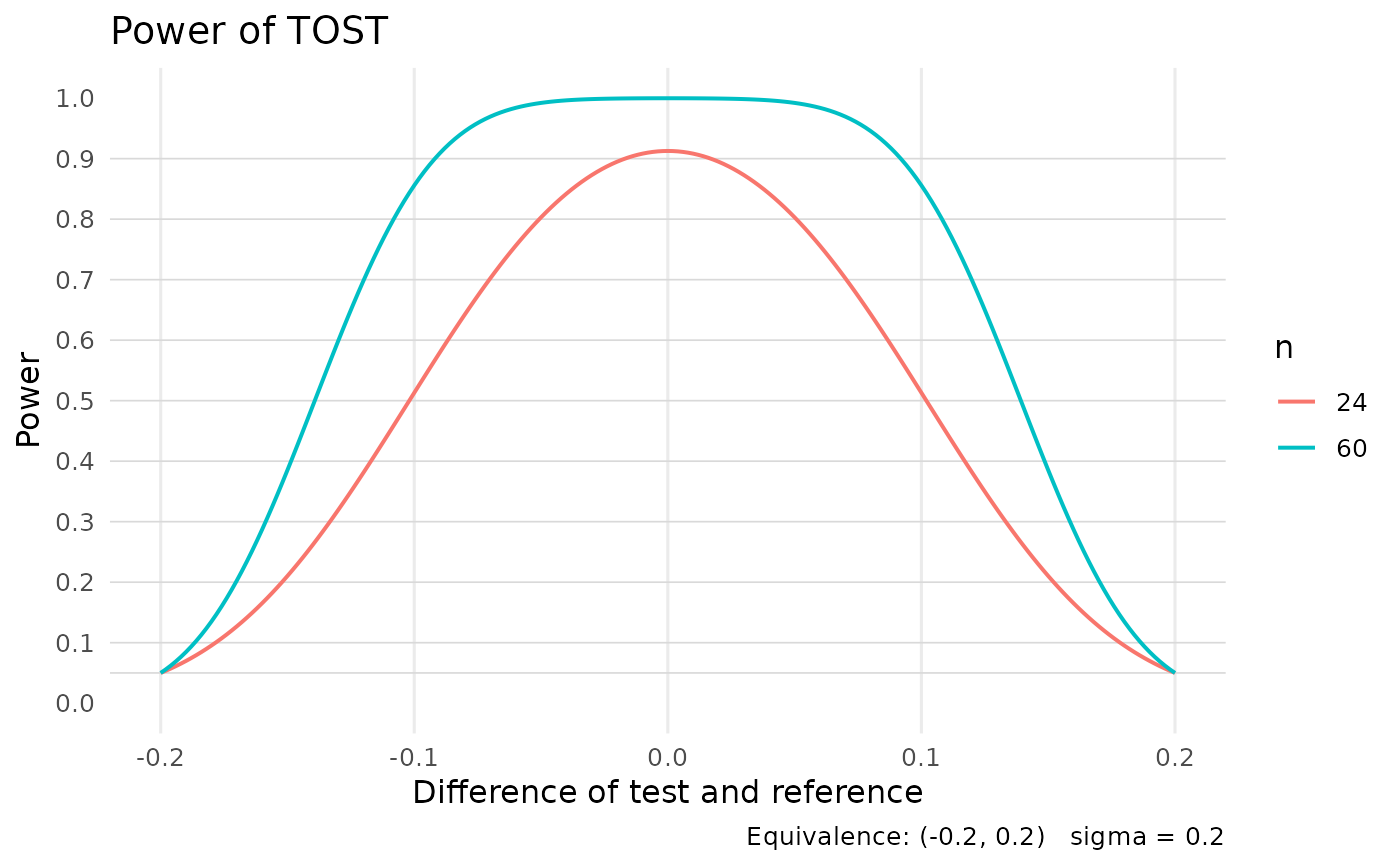
For each sample size in n, draws power as a function of the true mean difference (or ratio, on the log scale), evaluated at 201 equally spaced points across the equivalence interval. Returns a ggplot2 object; the underlying numerical grid is attached as attr(<plot>, "power_grid").

Usage

power_equivalence_md_plot(
  alpha_level,
  logscale,
  theta1,
  theta2,
  sigma,
  n,
  nu,
  title = NULL,
  subtitle = NULL
)

Arguments

alpha_level: Type I error rate for each of the two one-sided tests.
logscale: Logical. If TRUE, the means are compared on the logarithmic scale.
theta1: Lower limit of the equivalence interval.
theta2: Upper limit of the equivalence interval.
sigma: \(\sqrt{\mathrm{error\ variance}}\).
n: Vector of sample sizes (one curve per element).
nu: Vector of degrees of freedom for sigma, the same length as n.
title: Optional plot title (default "Power of TOST").
subtitle: Optional subtitle (typically a reference like "Phillips, Figure 3").

Value

A ggplot object. The 201-row power grid (column 1: true difference; remaining columns: power for each n) is attached as attr(<plot>, "power_grid").

Note

See the legacy MBESS package (Kelley, 2007a, 2007b) for additional details and discussion.

References

Diletti, E., Hauschke, D., & Steinijans, V. W. (1991). Sample size determination of bioequivalence assessment by means of confidence intervals. International Journal of Clinical Pharmacology, Therapy and Toxicology, 29(1), 1–8.

Kelley, K. (2007a). Confidence intervals for standardized effect sizes: Theory, application, and implementation. Journal of Statistical Software, 20(8), 1–24. doi:10.18637/jss.v020.i08

Kelley, K. (2007b). Methods for the behavioral, educational, and social sciences: An R package. Behavior Research Methods, 39(4), 979–984. doi:10.3758/BF03192993

Phillips, K. F. (1990). Power of the two one-sided tests procedure in bioequivalence. Journal of Pharmacokinetics and Biopharmaceutics, 18(2), 139–144. doi:10.1007/BF01063556

Schuirmann, D. J. (1987). A comparison of the two one-sided tests procedure and the power approach for assessing the equivalence of average bioavailability. Journal of Pharmacokinetics and Biopharmaceutics, 15(6), 657–680.

Author

Ken Kelley kkelley@nd.edu

Examples

# One curve per sample size, showing power against the true mean
# difference. Two of the seven sample sizes behind Phillips (1990)
# Figure 3 are drawn here so the example stays quick; the full
# reproduction is given below.
fig <- power_equivalence_md_plot(
  alpha_level = .05, logscale = FALSE,
  theta1 = -.2, theta2 = .2, sigma = .20,
  n = c(24, 60), nu = c(22, 58)
)
fig


# The numbers behind the curves travel with the figure, so a particular
# power value can be read off rather than eyeballed. The first column is
# the true difference and the remaining columns give power, one column
# per sample size. Power is highest where the true difference is zero.
power_grid <- attr(fig, "power_grid")
power_grid[which.min(abs(power_grid[, 1])), ]
#>      diff      n=24      n=60 
#> 0.0000000 0.9127046 0.9998349 

# The two published figures are not run here because every curve
# evaluates the power integral at 201 true differences, so a
# seven-curve figure costs a few tenths of a second. Phillips (1990)
# Figure 3 is:
# n  <- c(9, 12, 18, 24, 30, 40, 60)
# nu <- c(7, 10, 16, 22, 28, 38, 58)
# power_equivalence_md_plot(
#   alpha_level = .05, logscale = FALSE,
#   theta1 = -.2, theta2 = .2, sigma = .20,
#   n = n, nu = nu,
#   subtitle = "Phillips Figure 3"
# )

# Diletti (1991) Figure 1c is the same idea on the log scale, where the
# equivalence limits are the 0.80 to 1.25 ratio bounds used in
# bioequivalence work:
# n_d  <- c(8, 12, 18, 24, 30, 40, 60)
# nu_d <- c(6, 10, 16, 22, 28, 38, 58)
# power_equivalence_md_plot(
#   alpha_level = .05, logscale = TRUE,
#   theta1 = .8, theta2 = 1.25, sigma = .20,
#   n = n_d, nu = nu_d,
#   subtitle = "Diletti, Figure 1c"
# )