Plot Contrasts Against an Equivalence Region

Draws a forest-style plot of one or more contrast estimates with their 100(1 - 2\(\alpha\))% confidence intervals against the equivalence region \((-\delta_L, \delta_U)\) and the noninferiority bound \(-\delta_L\), colored by the five-way verdict of equivalence_c: an interval entirely inside the region is equivalent; entirely above \(\delta_U\), superior; entirely below \(-\delta_L\), inferior; a lower limit above \(-\delta_L\) with an upper limit past \(\delta_U\), noninferior only; and an interval straddling a bound, inconclusive. The geometry is the decision rule, which is what makes the plot the natural report of an equivalence analysis.

Usage

plot_equivalence(
  x = NULL,
  estimate = NULL,
  lower = NULL,
  upper = NULL,
  names = NULL,
  delta_lower = NULL,
  delta_upper = NULL,
  xlab = "Contrast",
  title = NULL,
  palette = "okabe_ito"
)

Arguments

x

Either a single result from equivalence_c or a list of them (a named list supplies the row labels). Alternatively, supply estimate, lower, and upper directly.

estimate, lower, upper

Numeric vectors of contrast estimates and their confidence limits, used when x is not supplied.

names

Optional character vector of row labels.

delta_lower, delta_upper

Equivalence bounds, as positive magnitudes (the region drawn is \((-\delta_L, +\delta_U)\)). Taken from x when it carries equivalence_c results; required otherwise. If only delta_upper is supplied, the bounds are symmetric.

xlab

The horizontal axis label. Default "Contrast".

title

Optional plot title.

palette

Character string naming the color palette for the verdict colors. Defaults to "okabe_ito", base R's colorblind-safe Okabe-Ito palette; "tableau" is also available.

Value

A ggplot object. Requires ggplot2 to be installed.

Details

The shaded band is the equivalence region and the dashed vertical lines are its bounds; the solid line at zero marks exact equality, which is the null value of ordinary significance testing and is deliberately not a decision boundary here. Verdicts are recomputed from the supplied limits and bounds, so the plot cannot disagree with equivalence_c.

References

Chattopadhyay, B., Bandyopadhyay, T., Kelley, K., & Padalunkal, J. J. (2025). A sequential approach for noninferiority or equivalence of a linear contrast under cost constraints. Psychological Methods, 30(2), 425–439. doi:10.1037/met0000570

Schuirmann, D. J. (1987). A comparison of the two one-sided tests procedure and the power approach for assessing the equivalence of average bioavailability. Journal of Pharmacokinetics and Biopharmaceutics, 15(6), 657–680.

See also

equivalence_c, plot_ci

Other equivalence testing: equivalence_c(), equivalence_r(), equivalence_smd(), power_density_equivalence_md(), power_equivalence_c(), power_equivalence_md(), power_equivalence_md_plot(), ss_power_equivalence_c()

Other plotting: plot_R2(), plot_cfa_k(), plot_ci(), plot_forest(), plot_irt_information(), plot_mediation_mbco(), plot_randomization_test(), plot_regions_of_significance(), plot_smd(), plot_trajectories(), plot_trajectories_fitted(), power_equivalence_md_plot()

Author

Ken Kelley kkelley@nd.edu

Examples

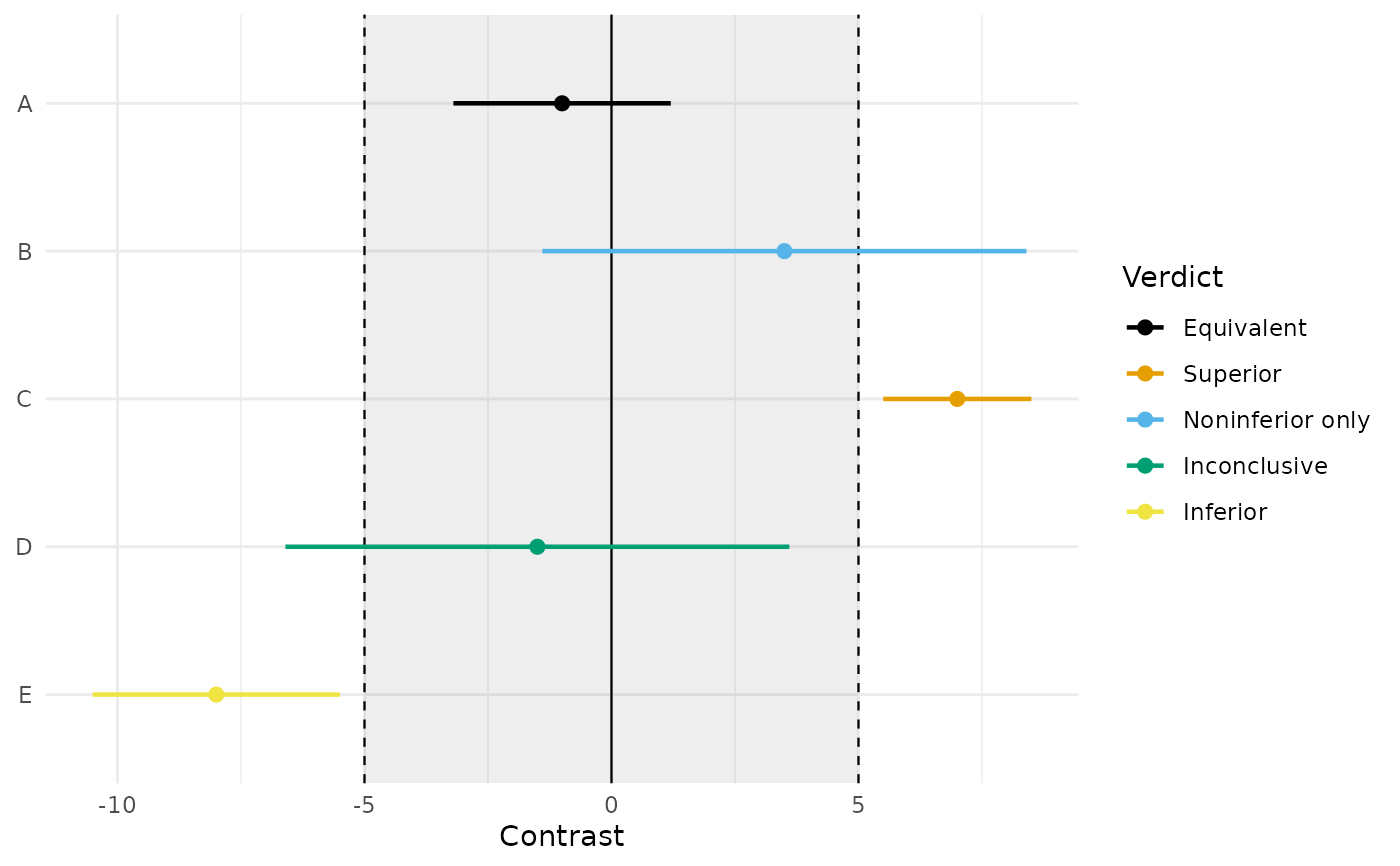
# Five constructed intervals, one per verdict, against bounds of 5
# (A equivalent, B noninferior only, C superior, D inconclusive,
#  E inferior):
plot_equivalence(estimate = c(-1.0, 3.5, 7.0, -1.5, -8.0),
                 lower    = c(-3.2, -1.4, 5.5, -6.6, -10.5),
                 upper    = c( 1.2,  8.4, 8.5,  3.6,  -5.5),
                 names    = c("A", "B", "C", "D", "E"),
                 delta_upper = 5)


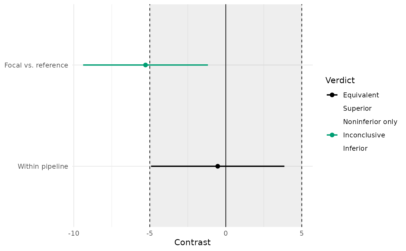
# From equivalence_c() results; a named list supplies the labels.
res <- list(
  "Focal vs. reference" = equivalence_c(psi_hat = -5.28, se = 2.49,
                                 df_error = 399, delta_upper = 5),
  "Within pipeline"     = equivalence_c(psi_hat = -0.53, se = 2.66,
                                 df_error = 399, delta_upper = 5)
)
plot_equivalence(res)