Plot an Item Response Theory Information Curve

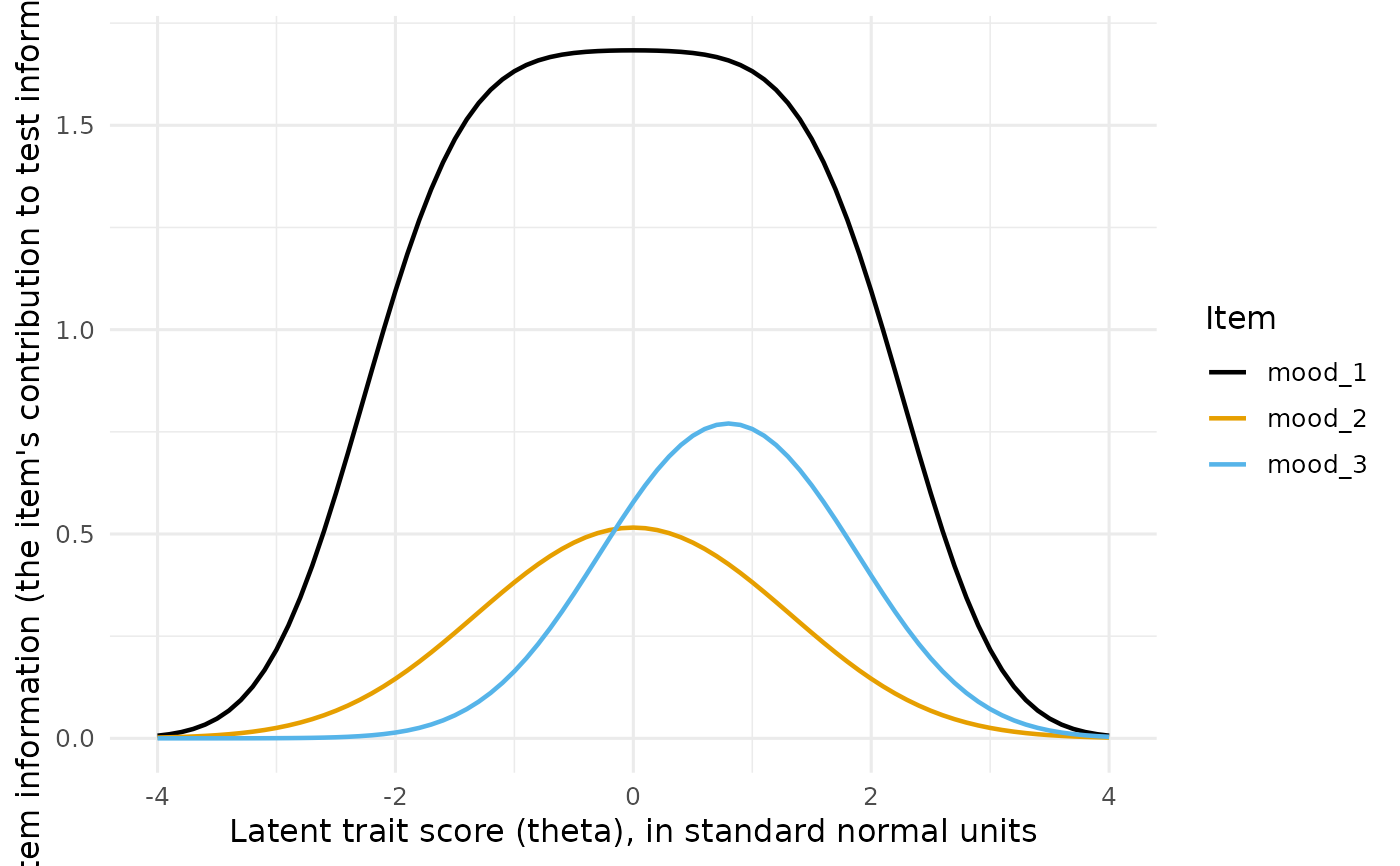
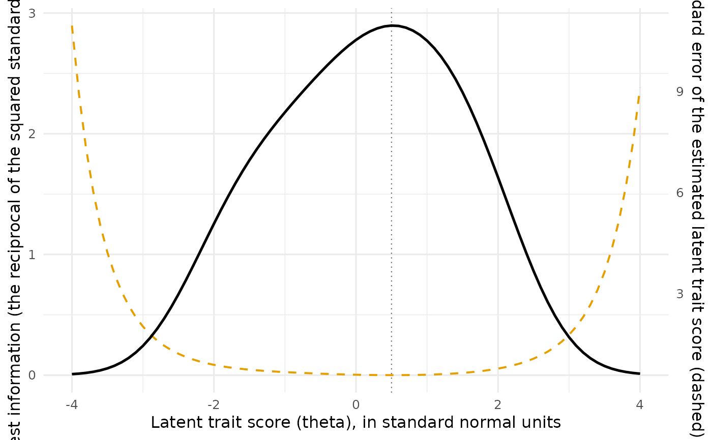
Draws the information function computed by irt_information: either the test information curve, with the standard error of the latent trait estimate on a secondary axis, or one curve per item. The test view answers "where on the latent continuum does this scale measure precisely?", and because the standard error is \(1 / \sqrt{I(\theta)}\) the same picture shows the precision directly. The item view decomposes that curve, since information is additive across items, and so shows which items cover which part of the continuum.

Usage

plot_irt_information(
  x,
  what = c("test", "item"),
  show_se = TRUE,
  show_peak = TRUE,
  palette = "okabe_ito",
  title = NULL,
  xlab = NULL,
  ylab = NULL
)

Arguments

x

The result of irt_information.

what

Which curves to draw: "test" (default) for the test information function, or "item" for one curve per item.

show_se

Logical. When TRUE (the default) and what = "test", the standard error of the latent trait estimate is drawn as a dashed curve against a secondary axis. The layer is omitted when the standard error is not finite and varying over the grid (for example when test information is zero somewhere).

show_peak

Logical. When TRUE (the default) and what = "test", a vertical dotted line marks the value of theta at which test information peaks on the supplied grid.

palette

Character string naming the color palette. Defaults to "okabe_ito", base R's colorblind-safe Okabe-Ito palette; "tableau" is also available.

title

Optional plot title.

xlab

Label for the horizontal axis. Defaults to a description of the latent trait metric.

ylab

Label for the vertical axis. Defaults to a description of the information plotted.

Value

A ggplot2 object.

Details

The secondary axis is a linear rescaling of the primary axis, so the dashed standard error curve shares the panel with the information curve without either being distorted relative to its own axis. The standard error is largest where information is smallest, which is why the two curves run in opposite directions.

Note

Requires ggplot2 (listed in Suggests).

References

Embretson, S. E., & Reise, S. P. (2000). Item response theory for psychologists. Lawrence Erlbaum.

Samejima, F. (1969). Estimation of latent ability using a response pattern of graded scores. Psychometrika Monograph Supplement, 34(4, Pt. 2), 1–97.

See also

irt_information

Other plotting: plot_R2(), plot_cfa_k(), plot_ci(), plot_equivalence(), plot_forest(), plot_mediation_mbco(), plot_randomization_test(), plot_regions_of_significance(), plot_smd(), plot_trajectories(), plot_trajectories_fitted(), power_equivalence_md_plot()

Author

Ken Kelley kkelley@nd.edu

Examples

info <- irt_information(
  a = c(mood_1 = 1.4, mood_2 = 0.9, mood_3 = 1.1),
  b = c(-1.5, -0.5, 0.5, 1.5, 0.0, 0.8),
  item = c(rep("mood_1", 4), "mood_2", "mood_3")
)

# Test information with the standard error on the secondary axis.
plot_irt_information(info)


# One curve per item.
plot_irt_information(info, what = "item")