Plot Observed and Fitted Individual Trajectories From a Multilevel Model

Given a fitted lme/nlme (nlme) or lmer (lme4) model, plots each subject's observed values and fitted curve on a smooth time grid, faceted one panel per subject. Per-subject \(R^2\) (squared correlation between observed and fitted values) and root-mean-square error are computed and attached to the returned ggplot2 object as the quality_of_fit attribute.

Usage

plot_trajectories_fitted(
  model,
  id = NULL,
  time = NULL,
  outcome = NULL,
  ids = NULL,
  n_random = NULL,
  pct_random = NULL,
  n_grid = 100,
  show_points = TRUE,
  point_size = 1.5,
  linewidth = 0.6,
  alpha = 0.8,
  palette = "okabe_ito",
  nrow = NULL,
  ncol = NULL,
  show_quality = TRUE,
  title = NULL,
  xlab = NULL,
  ylab = NULL,
  seed = NULL
)

Arguments

model: A fitted model object of class lme, nlme, or lmerMod.
id, time, outcome: Optional character names of the ID, time, and outcome columns. When NULL (the default), each is auto-detected from the model object: the outcome is the response variable in the formula, the ID is the first random-effect grouping factor, and time is the first fixed-effect predictor. Override these when the auto-detection is wrong.
ids, n_random, pct_random: Subject-subsetting options identical to those of plot_trajectories; at most one may be supplied.
n_grid: Integer. Number of points used to draw each subject's smooth fitted curve (default 100).
show_points: Logical. Whether to draw the observed values (default TRUE).
point_size, linewidth, alpha, nrow, ncol: Visual / layout controls.
palette: Character string naming the color palette; the fitted curve is drawn in the palette's primary color. Defaults to "okabe_ito", base R's colorblind-safe Okabe-Ito palette; "tableau" is also available.
show_quality: Logical. If TRUE (the default), each panel strip text includes the subject's \(R^2\) and RMSE.
title, xlab, ylab: Optional plot labels.
seed: Optional integer random seed used when n_random or pct_random is supplied. Defaults to NULL, which leaves the user's current RNG state intact; supply an integer for reproducible subject sampling.

Value

A ggplot object. The per-subject quality-of-fit data.frame (columns: id column, r_squared, rmse) is attached as attr(<plot>, "quality_of_fit").

Details

Modernizes the original vit_fitted() function by:

returning a ggplot2 object instead of writing to graphics devices,
attaching per-subject quality-of-fit as an attribute rather than assigning it to the global environment via <<- (a serious side effect of the original),
drawing a smooth fitted curve from a per-subject time grid via predict(..., re.form = NULL) for lme4 fits and predict(..., level = 1) for nlme fits,
correctly identifying lme4 fits (which use class lmerMod, not lmer).

Note

Requires ggplot2 plus, depending on the model class, nlme or lme4 (Suggests dependencies).

Author

Ken Kelley kkelley@nd.edu

Examples

# nlme: linear growth in tooth distance over age (Orthodont, 27 children).
# Four of the children are paneled here so the figure is quick to draw;
# drop n_random to get a panel for every child.
fm_nlme <- nlme::lme(distance ~ age, random = ~ age | Subject,
                     data = nlme::Orthodont)
p <- plot_trajectories_fitted(fm_nlme, n_random = 4, seed = 113)
p

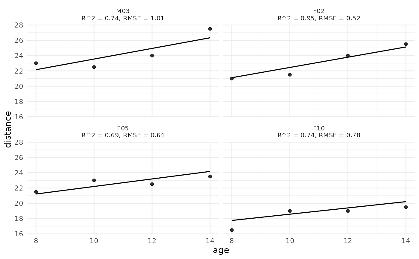attr(p, "quality_of_fit")  # per-subject R^2 and RMSE
#>   Subject r_squared      rmse
#> 1     M03 0.7377049 1.0072738
#> 2     F02 0.9481481 0.5232407
#> 3     F05 0.6914286 0.6397144
#> 4     F10 0.7363636 0.7785559

# An lme4 fit is handled the same way. Not run here because the call
# loads the lme4 namespace and then draws a panel for each of the
# eighteen subjects, which is where the time goes; fitting the model
# is quick by comparison. The calls are:
# fm_lme4 <- lme4::lmer(Reaction ~ Days + (Days | Subject),
#                       data = lme4::sleepstudy)
# plot_trajectories_fitted(fm_lme4)