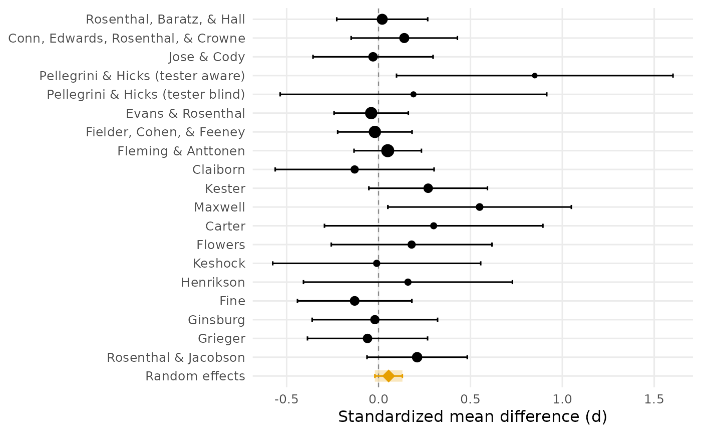
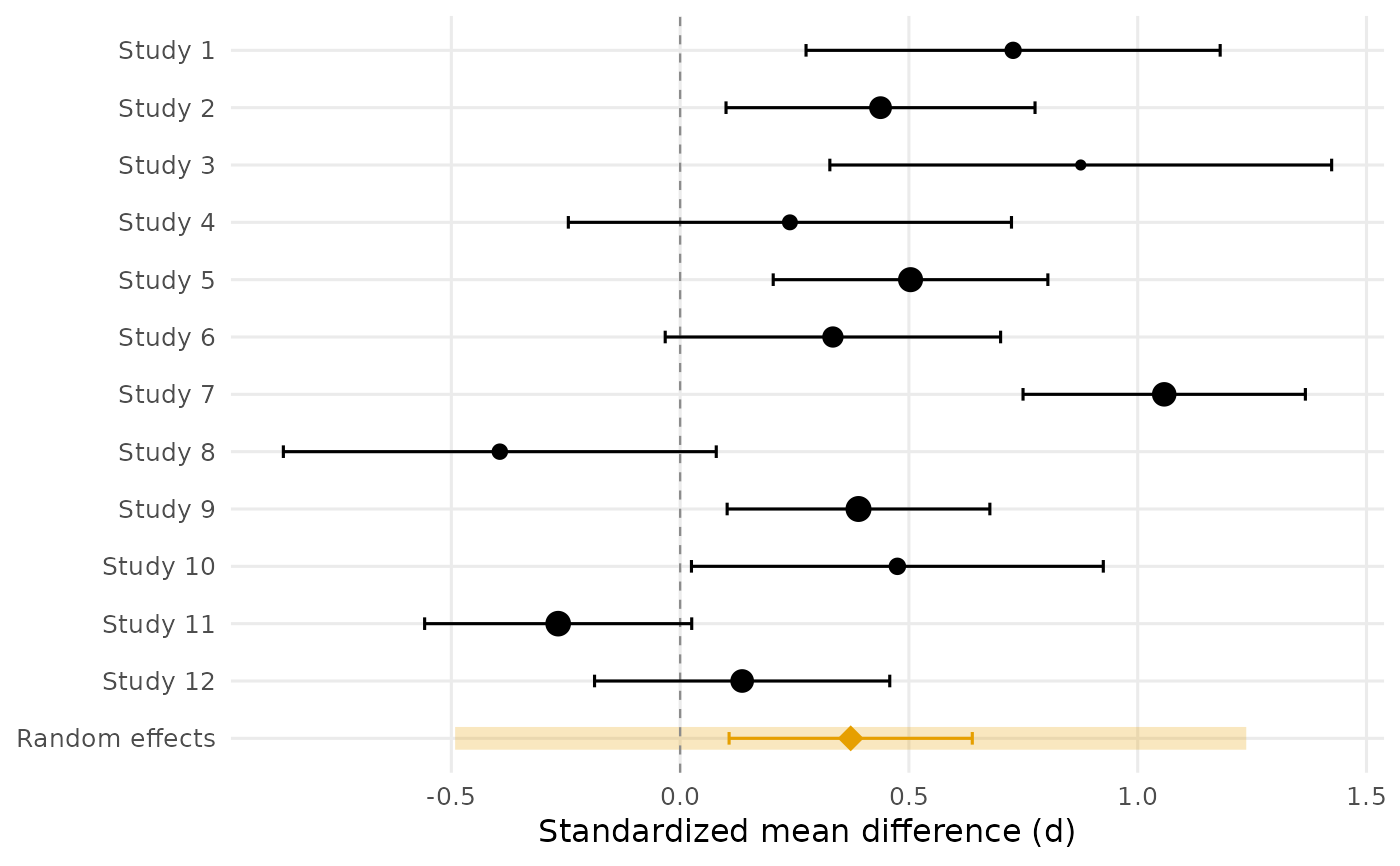
Draws the meta-analyst's central picture: every study's effect size with its confidence interval, the random effects pooled estimate beneath them, and, by default, the prediction interval showing where the effect of a new study is expected to land. Point sizes are proportional to precision (inverse variance), so the eye weighs the studies the way the model does. Requires ggplot2.
Usage
plot_forest(
  yi,
  vi,
  labels = NULL,
  method = c("reml", "pm", "dl", "fe"),
  hartung_knapp = TRUE,
  conf_level = 0.95,
  show_prediction = TRUE,
  xlab = "Effect size",
  title = NULL,
  palette = "okabe_ito",
  colors = NULL
)
Arguments
- yi
Numeric vector of study effect sizes.
- vi
Sampling variances of
yi.- labels
Optional study labels, one per study; defaults to
"Study 1","Study 2", and so on, in the supplied order.- method, hartung_knapp
Passed to
meta_esfor the pooled row ("reml"andTRUEby default).- conf_level
Confidence level for the per-study and pooled intervals. Defaults to 0.95.
- show_prediction
Logical: draw the prediction interval band on the pooled row? Default
TRUE(ignored formethod = "fe", which has none).- xlab
Label for the effect size axis. Defaults to
"Effect size".- title
Optional plot title.
- palette
Palette name. Defaults to
"okabe_ito", base R's colorblind-safe Okabe-Ito palette;"tableau"is also available.- colors
Optional length-2 vector overriding the palette: the study color and the pooled-estimate color.
See also
meta_es, meta_smd, and
meta_r for the numbers behind the picture;
teacher_expectancy for the example data.
Other meta-analysis:
combine_p(),
meta_contrast(),
meta_es(),
meta_r(),
meta_smd()
Other plotting:
plot_R2(),
plot_cfa_k(),
plot_ci(),
plot_equivalence(),
plot_irt_information(),
plot_mediation_mbco(),
plot_randomization_test(),
plot_regions_of_significance(),
plot_smd(),
plot_trajectories(),
plot_trajectories_fitted(),
power_equivalence_md_plot()
Author
Ken Kelley kkelley@nd.edu
Examples
# Twelve simulated studies whose true effects vary from study to study
# (between-study standard deviation 0.35), so the prediction interval
# for the effect of a new study is visibly wider than the confidence
# interval for the mean effect.
set.seed(113)
k <- 12
n <- sample(20:100, k) # per-group sample sizes
theta <- rnorm(k, mean = 0.4, sd = 0.35) # true study effects
d <- rnorm(k, mean = theta, sd = sqrt(2 / n))
v <- 2 / n + d^2 / (4 * n)
plot_forest(d, v, xlab = "Standardized mean difference (d)")
 # The teacher expectancy literature (Raudenbush, 1984): most studies
# cluster near zero, the estimated between-study variance is zero, and
# the prediction interval nearly coincides with the confidence interval.
data(teacher_expectancy)
d <- teacher_expectancy$d
n_e <- teacher_expectancy$n_experimental
n_c <- teacher_expectancy$n_control
v <- (n_e + n_c) / (n_e * n_c) + d^2 / (2 * (n_e + n_c))
plot_forest(d, v, labels = teacher_expectancy$author,
xlab = "Standardized mean difference (d)")
# The teacher expectancy literature (Raudenbush, 1984): most studies
# cluster near zero, the estimated between-study variance is zero, and
# the prediction interval nearly coincides with the confidence interval.
data(teacher_expectancy)
d <- teacher_expectancy$d
n_e <- teacher_expectancy$n_experimental
n_c <- teacher_expectancy$n_control
v <- (n_e + n_c) / (n_e * n_c) + d^2 / (2 * (n_e + n_c))
plot_forest(d, v, labels = teacher_expectancy$author,
xlab = "Standardized mean difference (d)")