Sample Size or Composite Power for a Factorial ANOVA
Source:R/ss_power_composite_factorial_anova.R
ss_power_composite_factorial_anova.RdDetermine the necessary per-cell sample size to achieve a desired level of
composite statistical power in a balanced factorial analysis of variance, or,
given a per-cell sample size, return the realized composite power. Composite
power is the probability that every effect named in effects is
statistically significant in the same study, the quantity a design must be
planned against when its conclusion requires more than one result to hold at
once.
Usage
ss_power_composite_factorial_anova(
  factor_levels,
  effects,
  means = NULL,
  sigma = NULL,
  desired_power = 0.85,
  alpha_level = 0.05,
  n_per_cell = NULL
)
Arguments
- factor_levels
Integer vector of the number of levels of each factor, one entry per factor (each at least 2). A
c(2, 3, 2)argument is a 2 by 3 by 2 design.- effects
A non-empty list naming the effects in the composite; see
ss_power_composite_factorial_ancovafor the format. Each element gives thefactorsan effect spans and itsforpartial_eta_squared, unlessmeansis supplied.- means
Optional array of population cell means (dimensions
factor_levels), or a numeric vector of lengthprod(factor_levels)in array order, from which each effect's Cohen's f is read givensigma. When supplied,plot()draws the mean pattern. Seess_power_composite_factorial_ancova.- sigma
The common within-cell standard deviation of the outcome, required with
meansand used only there.- desired_power
Desired composite statistical power (default 0.85). Used only when
n_per_cellisNULL.- alpha_level
Type I error rate for each individual F test (default 0.05), the per-test rate rather than a rate for the composite event.
- n_per_cell
Per-cell sample size, assumed balanced; if supplied, the realized composite power is returned rather than a sample size planned.
Value
A data.frame with term and value columns, as
ss_power_composite_factorial_ancova returns but with
covariate_R2 0 and n_covariates 0. It carries the
dmar_ss_power class for tidy /
glance and the
dmar_composite_power_factorial class for plot().
Details
This is the no-covariate case of ss_power_composite_factorial_ancova,
named directly. It does not take a covariate; when a covariate belongs in the
model, use ss_power_composite_factorial_ancova, which raises
every effect's power for the variance the covariate explains. With no
covariate the composite is exact to quadrature precision, since the balanced
factorial F tests are exactly noncentral F and exactly
independent given the shared error estimate.
See ss_power_composite_factorial_ancova for the model, the
one-dimensional integral that evaluates the composite over the shared error
estimate, and the figure the plot() method draws. Naming one effect
reproduces ss_power_factorial_anova exactly.
References
Maxwell, S. E. (2004). The persistence of underpowered studies in psychological research: Causes, consequences, and remedies. Psychological Methods, 9, 147–163.
Maxwell, S. E., Delaney, H. D., & Kelley, K. (2027). Designing experiments and analyzing data: A model comparison perspective (4th ed.). Routledge. (See Chapter 7 on factorial designs and Chapter 3 on statistical power.)
See also
ss_power_composite_factorial_ancova for the version
that admits a covariate; ss_power_factorial_anova for a single
effect
Other sample size for power:
power_fisher_exact(),
ss_aipe_mixed_effects(),
ss_power_R2(),
ss_power_R2_sensitivity(),
ss_power_c(),
ss_power_c_ancova(),
ss_power_composite_ancova(),
ss_power_composite_ancova_2group(),
ss_power_composite_anova(),
ss_power_composite_factorial_ancova(),
ss_power_composite_factorial_ancova_het(),
ss_power_composite_sem(),
ss_power_contrast(),
ss_power_equivalence_c(),
ss_power_factorial_ancova(),
ss_power_factorial_anova(),
ss_power_indirect_effect(),
ss_power_mixed_effects(),
ss_power_one_way_anova(),
ss_power_pcm(),
ss_power_r(),
ss_power_rc(),
ss_power_reg_coef(),
ss_power_reg_coef_sensitivity(),
ss_power_rm_anova(),
ss_power_sc(),
ss_power_sem(),
ss_power_smd(),
ss_power_split_plot_anova()
Other composite power:
ss_power_composite_ancova(),
ss_power_composite_ancova_2group(),
ss_power_composite_anova(),
ss_power_composite_factorial_ancova(),
ss_power_composite_factorial_ancova_het(),
ss_power_composite_sem()
Author
Ken Kelley kkelley@nd.edu
Examples
# A 2 by 3 factorial ANOVA whose conclusion needs both main effects. Plan
# against their composite, not against either one alone.
ss_power_composite_factorial_anova(
factor_levels = c(2, 3),
effects = list(list(factors = 1, f = 0.25),
list(factors = 2, f = 0.20)),
desired_power = 0.80)
#> term value
#> necessary_n_per_cell 43
#> necessary_N 258
#> composite_power 0.806
#> residual_df 252
#> power_1 0.979
#> power_2 0.823
#> f_1 0.25
#> f_2 0.2
#> df_1 1
#> df_2 2
#> noncentral_parm_1 16.1
#> noncentral_parm_2 10.3
#> covariate_R2 0
#> n_covariates 0
#> cells 6
#> alpha_level 0.05
#> desired_power 0.8
# Realized composite power at 25 per cell for a main effect and the
# three-way interaction of a 2 by 2 by 2 design.
ss_power_composite_factorial_anova(
factor_levels = c(2, 2, 2),
effects = list(list(factors = 1, f = 0.30, label = "A"),
list(factors = c(1, 2, 3), f = 0.25, label = "AxBxC")),
n_per_cell = 25)
#> term value
#> specified_n_per_cell 25
#> specified_N 200
#> composite_power 0.929
#> residual_df 192
#> power_A 0.988
#> power_AxBxC 0.94
#> f_A 0.3
#> f_AxBxC 0.25
#> df_A 1
#> df_AxBxC 1
#> noncentral_parm_A 18
#> noncentral_parm_AxBxC 12.5
#> covariate_R2 0
#> n_covariates 0
#> cells 8
#> alpha_level 0.05
# Naming one effect reproduces the single-effect planner exactly.
ss_power_composite_factorial_anova(
factor_levels = c(2, 3), effects = list(list(factors = 2, f = 0.25)),
n_per_cell = 20)
#> term value
#> specified_n_per_cell 20
#> specified_N 120
#> composite_power 0.675
#> residual_df 114
#> power_2 0.675
#> f_2 0.25
#> df_2 2
#> noncentral_parm_2 7.5
#> covariate_R2 0
#> n_covariates 0
#> cells 6
#> alpha_level 0.05
ss_power_factorial_anova(factor_levels = c(2, 3), effect_indices = 2,
f = 0.25, n_per_cell = 20)
#> term value
#> specified_n_per_cell 20
#> total_N 120
#> effect_df 2
#> error_df 114
#> noncentrality 7.5
#> actual_power 0.675
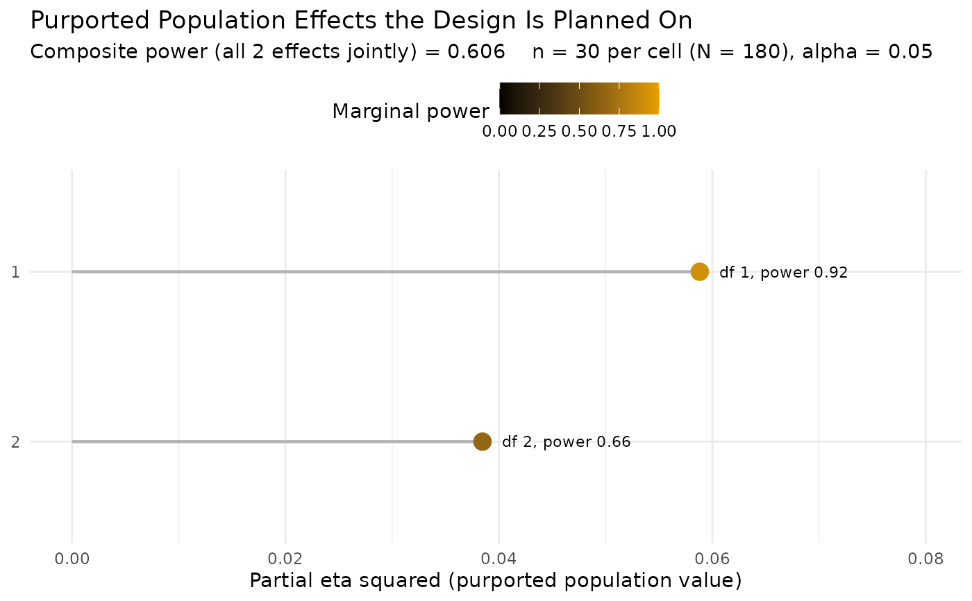
# The figure of the purported population effect sizes.
plot(ss_power_composite_factorial_anova(
factor_levels = c(2, 3),
effects = list(list(factors = 1, f = 0.25),
list(factors = 2, f = 0.20)),
n_per_cell = 30))
 # Stating the effects as population cell means with a common within-cell SD.
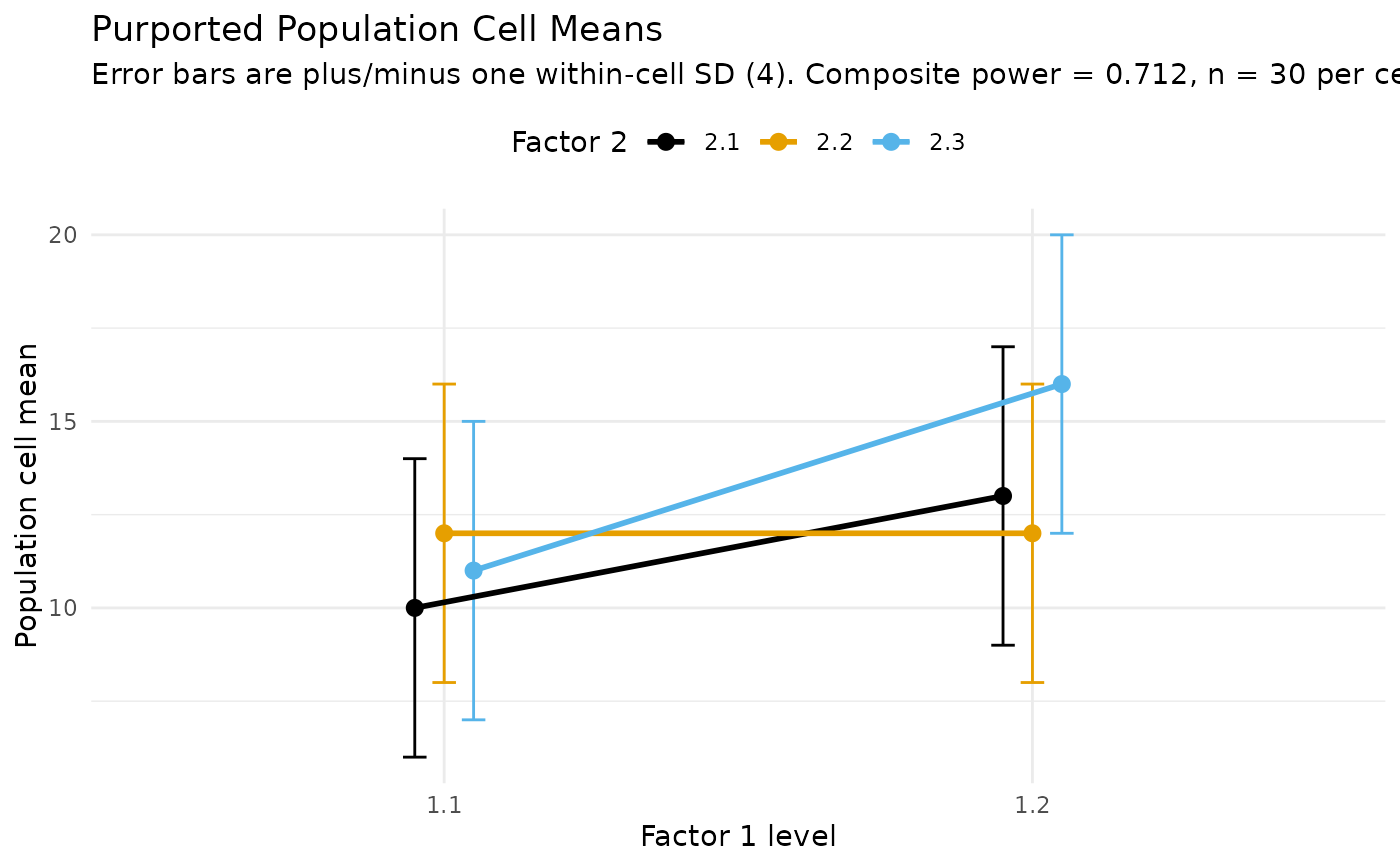
# plot() then draws the mean pattern, with error bars of one SD.
cell_means <- matrix(c(10, 12, 11,
13, 12, 16), nrow = 2, byrow = TRUE)
plot(ss_power_composite_factorial_anova(
factor_levels = c(2, 3), means = cell_means, sigma = 4,
effects = list(list(factors = 1, label = "A"),
list(factors = 2, label = "B")),
n_per_cell = 30))
# Stating the effects as population cell means with a common within-cell SD.
# plot() then draws the mean pattern, with error bars of one SD.
cell_means <- matrix(c(10, 12, 11,
13, 12, 16), nrow = 2, byrow = TRUE)
plot(ss_power_composite_factorial_anova(
factor_levels = c(2, 3), means = cell_means, sigma = 4,
effects = list(list(factors = 1, label = "A"),
list(factors = 2, label = "B")),
n_per_cell = 30))