Sample Size or Composite Power for a One-Way or Factorial ANCOVA

Determine the necessary per-cell sample size to achieve a desired level of composite statistical power in a balanced analysis of covariance with \(a\) groups (a one-way design) or a factorial arrangement of factors, or, given a per-cell sample size, return the realized composite power. Composite power is the probability that every effect named in effects is statistically significant in the same study, the quantity a design must be planned against when its conclusion requires more than one result to hold at once.

Usage

ss_power_composite_ancova(
  factor_levels,
  effects,
  slopes = c("homogeneous", "heterogeneous"),
  means = NULL,
  sigma = NULL,
  covariate_R2 = 0,
  n_covariates = 0,
  correlations = NULL,
  sd_cov = 1,
  desired_power = 0.85,
  alpha_level = 0.05,
  n_per_cell = NULL
)

Arguments

factor_levels: Integer vector of the number of levels of each factor, one entry per factor (each at least 2). A single value a is a one-way design with \(a\) groups; c(2, 3) is a 2 by 3 factorial.
effects: A non-empty list naming the effects in the composite. For slopes = "homogeneous" each element has factors (the factor indices the effect spans) and, unless means is supplied, its effect size f or partial_eta_squared. For slopes = "heterogeneous" each element also has a type, one of "mean" (a factorial mean effect, the default), "covariate" (the average slope, spanning no factors), or "slope" (a factor-by-covariate slope heterogeneity). An optional label names the effect. See the forwarded functions for the exact grammar.
slopes: The covariate-slope model, "homogeneous" (one common slope, the default) or "heterogeneous" (the slope may differ across cells, making the covariate and slope-heterogeneity effects testable).
means: Optional array of population cell means (dimensions factor_levels, or a vector in array order) from which the mean effects' sizes are read; enables the mean-pattern figure.
sigma: The common within-cell population standard deviation of the outcome, required with the population-values interface.
covariate_R2: For slopes = "homogeneous" only: proportion of the outcome's within-cell variance the covariate or covariates explain, in \([0, 1)\), which raises every effect's noncentrality through \(f / \sqrt{1 - R^2}\). Defaults to 0.
n_covariates: For slopes = "homogeneous" only: number of covariates, each spending one residual degree of freedom. Must be positive when covariate_R2 is. Defaults to 0.
correlations: For slopes = "heterogeneous" only: optional array of the population covariate-outcome correlation within each cell (dimensions factor_levels), which supplies the covariate and slope effects' sizes with the population-values interface.
sd_cov: For slopes = "heterogeneous" only: population standard deviation of the covariate, the units the slopes and the figure are drawn in. Scale free, so it changes no power. Default 1.
desired_power: Desired composite statistical power (default 0.85). Used only when n_per_cell is NULL.
alpha_level: Type I error rate for each individual F test (default 0.05), the per-test rate, not a rate for the composite event.
n_per_cell: Per-cell sample size (balanced); if supplied, the realized composite power is returned rather than a sample size planned.

Value

The data.frame the forwarded planner returns, with term and value columns and the dmar_ss_power class for tidy and glance, plus the dmar_composite_power_factorial (homogeneous) or dmar_composite_power_factorial_het (heterogeneous) class for plot(). See ss_power_composite_factorial_ancova for the row-by-row description.

Details

This is the general entry point for the ANCOVA composite. The two-group design has its own simpler interface in ss_power_composite_ancova_2group, stated through a single smd and one or two correlations; use that when there are exactly two groups. Use this function for more than two groups or for a factorial design. With no covariate, name the effects through ss_power_composite_anova instead.

Homogeneous or heterogeneous slopes. The slopes argument chooses the model. "homogeneous" (the default) assumes one common covariate slope across the cells; the covariate is a variance reducer and the composite is over the factorial mean effects. "heterogeneous" lets the slope differ across cells, which makes the average covariate slope and the factor-by-covariate slope heterogeneity into testable effects that can join the mean effects in the composite. The heterogeneous one-way case is the \(a\)-group generalization of the two-group ANCOVA composite: a group mean effect, the covariate effect, and the group-by-covariate slope heterogeneity.

This function is a thin dispatcher. slopes = "homogeneous" forwards to ss_power_composite_factorial_ancova and slopes = "heterogeneous" to ss_power_composite_factorial_ancova_het; see those for the full method, the exactness discussion, and the shape of the returned object. The population effects can be stated as effect sizes or as population values (cell means, and for heterogeneous slopes a covariate-outcome correlation per cell) with a common within-cell standard deviation, from which the plot() method draws the population pattern.

References

Maxwell, S. E. (2004). The persistence of underpowered studies in psychological research: Causes, consequences, and remedies. Psychological Methods, 9, 147–163.

Maxwell, S. E., Delaney, H. D., & Kelley, K. (2027). Designing experiments and analyzing data: A model comparison perspective (4th ed.). Routledge. (See Chapter 9 on the analysis of covariance, Chapter 7 on factorial designs, and Chapter 3 on statistical power.)

Author

Ken Kelley kkelley@nd.edu

Examples

# A four-group (one-way) ANCOVA with heterogeneous slopes: the a-group
# generalization of the two-group composite. The conclusion needs the group
# mean effect, a covariate effect, and evidence that the covariate slope
# differs across the groups, so the design is planned against all three.
ss_power_composite_ancova(
  factor_levels = 4, slopes = "heterogeneous",
  effects = list(list(type = "mean",      factors = 1, f = 0.30),
                 list(type = "covariate",              f = 0.40),
                 list(type = "slope",      factors = 1, f = 0.20)),
  desired_power = 0.80)
#>  term                      value
#>  necessary_n_per_cell      71   
#>  necessary_N               284  
#>  composite_power           0.807
#>  residual_df               276  
#>  power_1                   0.994
#>  power_covariate           1    
#>  power_cov_x_1             0.812
#>  f_1                       0.3  
#>  f_covariate               0.4  
#>  f_cov_x_1                 0.2  
#>  df_1                      3    
#>  df_covariate              1    
#>  df_cov_x_1                3    
#>  noncentral_parm_1         25.6 
#>  noncentral_parm_covariate 45.4 
#>  noncentral_parm_cov_x_1   11.4 
#>  cells                     4    
#>  alpha_level               0.05 
#>  desired_power             0.8  

# A 2 by 3 factorial ANCOVA with one common slope. Both main effects must
# hold; the covariate explains 25 percent of the within-cell variance.
ss_power_composite_ancova(
  factor_levels = c(2, 3),
  effects = list(list(factors = 1, f = 0.25),
                 list(factors = 2, f = 0.20)),
  covariate_R2 = 0.25, n_covariates = 1,
  desired_power = 0.80)
#>  term                 value
#>  necessary_n_per_cell 32   
#>  necessary_N          192  
#>  composite_power      0.801
#>  residual_df          185  
#>  power_1              0.978
#>  power_2              0.818
#>  f_1                  0.25 
#>  f_2                  0.2  
#>  df_1                 1    
#>  df_2                 2    
#>  noncentral_parm_1    16   
#>  noncentral_parm_2    10.2 
#>  covariate_R2         0.25 
#>  n_covariates         1    
#>  cells                6    
#>  alpha_level          0.05 
#>  desired_power        0.8  

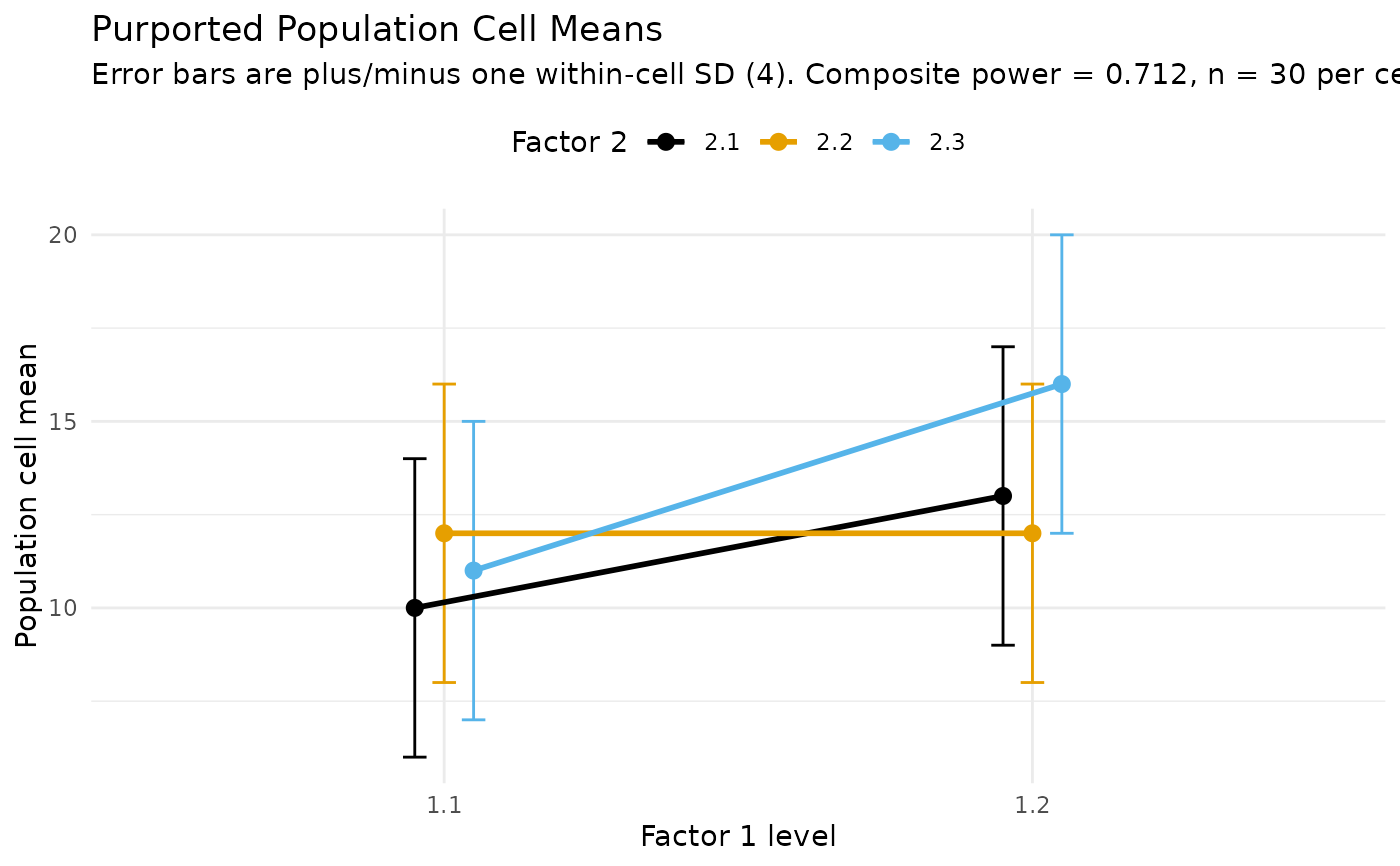
# The population effects can instead be a full pattern of cell means with a
# common within-cell SD; plot() then draws the mean pattern itself.
cell_means <- matrix(c(10, 12, 11,
                       13, 12, 16), nrow = 2, byrow = TRUE)
fit <- ss_power_composite_ancova(
  factor_levels = c(2, 3), means = cell_means, sigma = 4,
  effects = list(list(factors = 1, label = "A"),
                 list(factors = 2, label = "B")),
  n_per_cell = 30)
fit
#>  term                 value
#>  specified_n_per_cell 30   
#>  specified_N          180  
#>  composite_power      0.712
#>  residual_df          174  
#>  power_A              0.994
#>  power_B              0.717
#>  f_A                  0.333
#>  f_B                  0.212
#>  df_A                 1    
#>  df_B                 2    
#>  noncentral_parm_A    20   
#>  noncentral_parm_B    8.12 
#>  covariate_R2         0    
#>  n_covariates         0    
#>  cells                6    
#>  alpha_level          0.05 
plot(fit)


# A one-row broom summary of a plan.
generics::tidy(ss_power_composite_ancova(
  factor_levels = c(2, 3),
  effects = list(list(factors = 1, f = 0.25),
                 list(factors = 2, f = 0.20)),
  desired_power = 0.80))
#>          term estimate     power
#> 1 sample_size       43 0.8064647

# The two-group case matches the dedicated two-group planner. Here factor 1
# has two levels, so the heterogeneous one-way composite reproduces
# ss_power_composite_ancova_2group with one correlation per group.
ss_power_composite_ancova(
  factor_levels = 2, slopes = "heterogeneous",
  means = c(0, 0.5), correlations = c(0.1, 0.5), sigma = 1,
  effects = list(list(type = "mean", factors = 1),
                 list(type = "covariate"),
                 list(type = "slope", factors = 1)),
  n_per_cell = 95)
#> Warning: The cell correlations differ in absolute value, so the cells' residual variances differ and the shared-error composite power is an approximation whose error grows with the spread of the correlations. The powers are reported as approximate_* rows, and a planned sample size as approximate_n_per_cell, because neither is exact; confirm a final design by simulation.
#>  term                        value
#>  specified_n_per_cell        95   
#>  specified_N                 190  
#>  approximate_composite_power 0.795
#>  residual_df                 186  
#>  approximate_power_1         0.957
#>  approximate_power_covariate 0.993
#>  approximate_power_cov_x_1   0.837
#>  f_1                         0.268
#>  f_covariate                 0.322
#>  f_cov_x_1                   0.214
#>  df_1                        1    
#>  df_covariate                1    
#>  df_cov_x_1                  1    
#>  noncentral_parm_1           13.6 
#>  noncentral_parm_covariate   19.7 
#>  noncentral_parm_cov_x_1     8.74 
#>  cells                       2    
#>  alpha_level                 0.05 
ss_power_composite_ancova_2group(smd = 0.5, rho = c(0.1, 0.5), n = 95)
#> Warning: The group correlations differ in absolute value, so the groups' residual variances differ and the shared-error composite power is an approximation whose error grows with the gap between the correlations. The powers are reported as approximate_* rows, and a planned sample size as approximate_n_per_group, because neither is exact; confirm a final design by simulation.
#>  term                                 value
#>  specified_n_per_group                95   
#>  specified_N                          190  
#>  approximate_composite_power          0.795
#>  residual_df                          186  
#>  approximate_power_group              0.957
#>  approximate_power_covariate          0.993
#>  approximate_power_group_by_covariate 0.837
#>  noncentral_t_parm_group              3.69 
#>  noncentral_t_parm_covariate          4.43 
#>  noncentral_t_parm_group_by_covariate 2.96 
#>  supposed_smd                         0.5  
#>  supposed_rho_group_1                 0.1  
#>  supposed_rho_group_2                 0.5  
#>  sigma                                1    
#>  sd_cov                               1    
#>  alpha_level                          0.05 
#>  tails                                2