Sample Size or Composite Power for a Factorial ANCOVA

Determine the necessary per-cell sample size to achieve a desired level of composite statistical power in a balanced factorial analysis of covariance, or, given a per-cell sample size, return the realized composite power. Composite power is the probability that every effect named in effects is statistically significant in the same study, the quantity a design must be planned against when its conclusion requires more than one result to hold at once. Each effect is a main effect or an interaction of the factorial design, tested by its own F test, and any subset of them can make up the composite.

Usage

ss_power_composite_factorial_ancova(
  factor_levels,
  effects,
  means = NULL,
  sigma = NULL,
  covariate_R2 = 0,
  n_covariates = 0,
  desired_power = 0.85,
  alpha_level = 0.05,
  n_per_cell = NULL
)

# S3 method for class 'dmar_composite_power_factorial'
plot(x, ...)

Arguments

factor_levels: Integer vector of the number of levels of each factor, one entry per factor (each at least 2). A c(2, 3, 2) argument is a 2 by 3 by 2 design.
effects: A non-empty list naming the effects in the composite. Each element is itself a list with factors (a vector of factor indices into factor_levels: one index for a main effect, several for an interaction) and exactly one of f (Cohen's f for that effect) or partial_eta_squared. An optional label names the effect in the output and the figure; the default label is the factor indices joined by x (for example "1x2" for the interaction of factors 1 and 2). Each element also carries the effect size, one of f or partial_eta_squared, unless means is supplied, in which case the sizes come from the means and no effect size is given here. The purported effect sizes are population values the researcher posits, never sample estimates.
means: Optional array of population cell means whose dimensions are factor_levels (a matrix for two factors), or a numeric vector of length prod(factor_levels) in array order (the first factor varying fastest). When supplied, each named effect's Cohen's f is computed from the means and sigma, and plot() draws the mean pattern. The means are the population values the researcher posits, on the raw scale of the outcome.
sigma: The common within-cell population standard deviation of the outcome (the square root of the error variance), required with means and used only there. Cohen's f for an effect is the spread of its cell-mean component relative to sigma.
covariate_R2: Proportion of the outcome's within-cell variance the covariate or covariates explain, in \([0, 1)\). The covariate removes that fraction of the error variance, which raises every effect's noncentrality through \(f / \sqrt{1 - R^2}\). Defaults to 0.
n_covariates: Number of covariates, a non-negative integer. Each spends one residual degree of freedom. Must be positive when covariate_R2 is. Defaults to 0.
desired_power: Desired composite statistical power (default 0.85). Used only when n_per_cell is NULL.
alpha_level: Type I error rate for each individual F test (default 0.05). This is the per-test rate, not a rate for the composite event.
n_per_cell: Per-cell sample size, assumed balanced across cells; if supplied, the realized composite power is returned rather than a sample size planned.
x: An object returned by ss_power_composite_factorial_ancova or ss_power_composite_factorial_anova.
...: Further arguments to the figure: palette (a palette name, default "okabe_ito") and title.

Value

A data.frame with term and value columns: the recommended (or supplied) n_per_cell and total N, the composite_power, the residual_df, then for each effect its marginal power_<label>, purported f_<label>, numerator df_<label>, and noncentral_parm_<label>, followed by rows echoing covariate_R2, n_covariates, cells, and alpha_level. The result carries the dmar_ss_power class, so tidy and glance summarize the per-cell size and the composite power in broom convention, and a dmar_composite_power_factorial class so plot() draws the figure.

Details

The population effects can be stated two ways: as effect sizes, a Cohen's f or partial eta squared per effect, or as a full array of population cell means together with a common within-cell standard deviation, from which each named effect's f is read off the analysis of variance decomposition of the means. Supplying means lets the plot() method draw the mean pattern itself, so the size of the population effects is on the page.

With no covariate (the defaults covariate_R2 = 0 and n_covariates = 0) this is a factorial ANOVA; the wrapper ss_power_composite_factorial_anova is that case named directly.

In a balanced factorial design the effect sums of squares are mutually orthogonal, so the effects are uncorrelated. Orthogonal effects do not give independent tests: every F test divides by the same error mean square, so an error estimate that lands low inflates all of the test statistics together. The tests are positively dependent, and composite power is strictly larger than the product of the marginal powers, bounded above by the least powerful test in the set, so the weakest effect governs the design.

Conditional on the error estimate the tests are independent, which reduces the composite to a one dimensional integral over the chi square distribution of that estimate. Effect \(j\) has numerator degrees of freedom \(\prod (a - 1)\) over the factors it spans and noncentrality \(N f_{\mathrm{adj}}^2\) with \(f_{\mathrm{adj}} = f / \sqrt{1 - R^2}\) and \(N\) the total sample size, the same convention and covariate adjustment ss_power_factorial_ancova uses. The residual degrees of freedom are \(N - \mathrm{cells} - \mathrm{covariates}\). Adaptive quadrature evaluates the integral, so nothing is simulated and the result is deterministic to quadrature precision. A single-effect composite reproduces the ordinary noncentral F power, and naming one effect reproduces ss_power_factorial_anova (or ss_power_factorial_ancova with a covariate) exactly.

Exactness. With no covariate the composite is exact to quadrature precision: the balanced factorial F tests are exactly noncentral F and exactly independent given the error estimate. A covariate introduces the one approximation ss_power_factorial_ancova already carries, treating covariate_R2 as a fixed reduction of the error variance rather than an estimated one; the departure is of order \(1 / N\) and is negligible at the sample sizes a multi-effect composite usually needs.

Because every test divides by the same error estimate, composite power is not strictly monotone in n_per_cell at the smallest residual degrees of freedom. necessary_n_per_cell is the smallest per-cell size attaining desired_power.

Functions

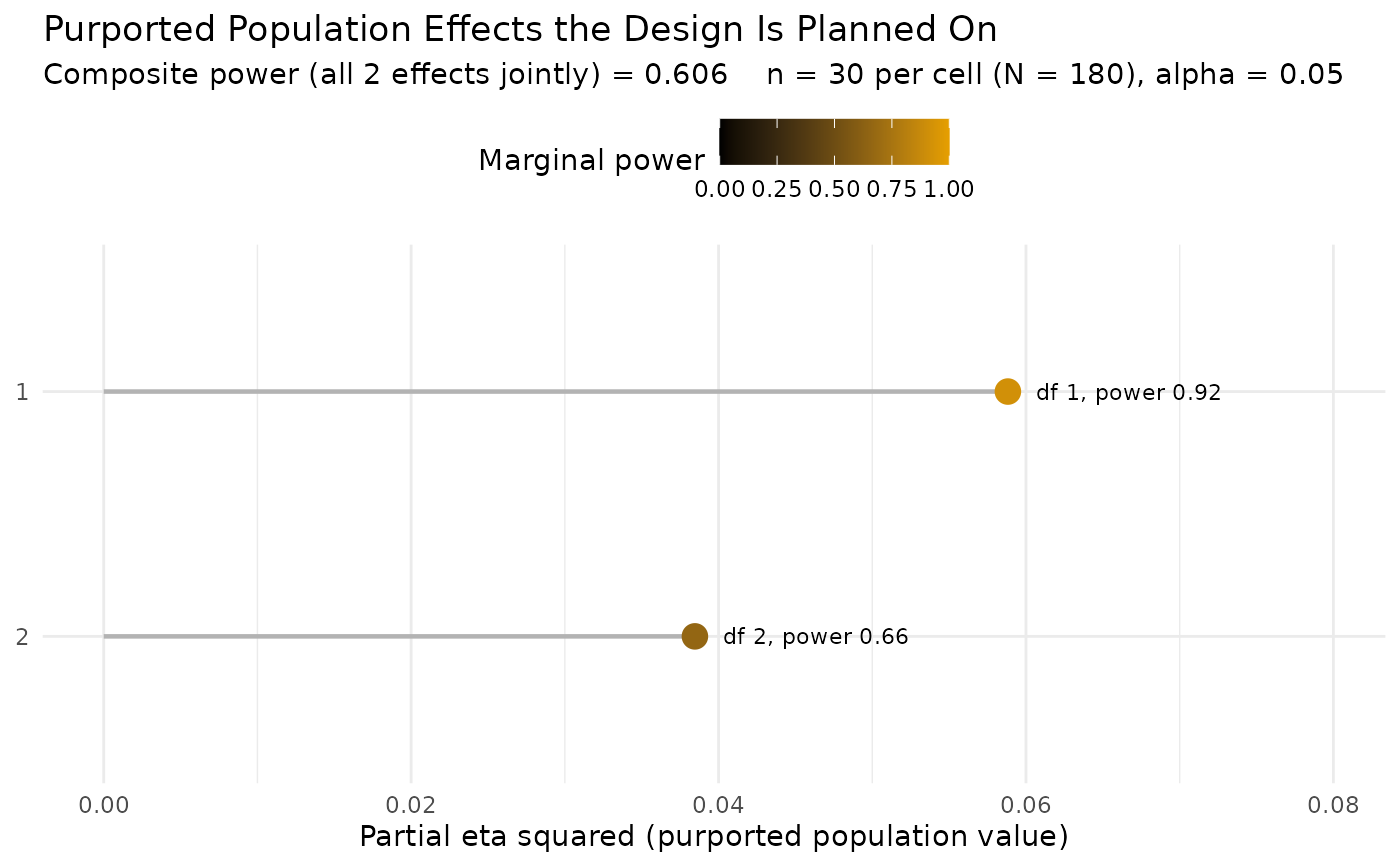
plot(dmar_composite_power_factorial): Draw the purported population effect sizes a result was planned on, each annotated with its marginal power, and the composite power in the subtitle.

The figure

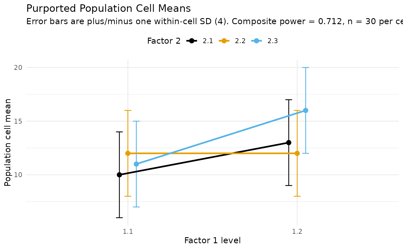
The plot() method draws the purported population values. When means were supplied it draws the mean pattern itself: a profile of the population cell means over the first factor, one line per level of the second, faceted by any further factors, with an error bar of plus or minus one within-cell standard deviation at each mean so the effect sizes read against the noise. When effect sizes were supplied instead, the cell means are not pinned (many mean patterns share one Cohen's f), so it draws the effect sizes: one lollipop per named effect at its partial eta squared, colored and labeled by that effect's marginal power. Either way the composite power is in the subtitle and nothing is simulated. Requires ggplot2.

References

Maxwell, S. E. (2004). The persistence of underpowered studies in psychological research: Causes, consequences, and remedies. Psychological Methods, 9, 147–163.

Maxwell, S. E., Delaney, H. D., & Kelley, K. (2027). Designing experiments and analyzing data: A model comparison perspective (4th ed.). Routledge. (See Chapter 7 on factorial designs, Chapter 9 on the analysis of covariance, and Chapter 3 on statistical power.)

Author

Ken Kelley kkelley@nd.edu

Examples

# A 2 by 3 factorial ANCOVA. The conclusion needs both main effects to hold,
# so the design is planned against their composite. The covariate explains
# 25 percent of the within-cell variance (one covariate).
ss_power_composite_factorial_ancova(
  factor_levels = c(2, 3),
  effects = list(list(factors = 1, f = 0.25),
                 list(factors = 2, f = 0.20)),
  covariate_R2 = 0.25, n_covariates = 1,
  desired_power = 0.80)
#>  term                 value
#>  necessary_n_per_cell 32   
#>  necessary_N          192  
#>  composite_power      0.801
#>  residual_df          185  
#>  power_1              0.978
#>  power_2              0.818
#>  f_1                  0.25 
#>  f_2                  0.2  
#>  df_1                 1    
#>  df_2                 2    
#>  noncentral_parm_1    16   
#>  noncentral_parm_2    10.2 
#>  covariate_R2         0.25 
#>  n_covariates         1    
#>  cells                6    
#>  alpha_level          0.05 
#>  desired_power        0.8  

# Realized composite power at 40 per cell for a main effect and the
# interaction of a 2 by 2 design, effect sizes given as partial eta squared.
ss_power_composite_factorial_ancova(
  factor_levels = c(2, 2),
  effects = list(list(factors = 1,        partial_eta_squared = 0.06),
                 list(factors = c(1, 2),  partial_eta_squared = 0.04)),
  n_per_cell = 40)
#>  term                 value
#>  specified_n_per_cell 40   
#>  specified_N          160  
#>  composite_power      0.647
#>  residual_df          156  
#>  power_1              0.888
#>  power_1x2            0.728
#>  f_1                  0.253
#>  f_1x2                0.204
#>  df_1                 1    
#>  df_1x2               1    
#>  noncentral_parm_1    10.2 
#>  noncentral_parm_1x2  6.67 
#>  covariate_R2         0    
#>  n_covariates         0    
#>  cells                4    
#>  alpha_level          0.05 

# Naming one effect reproduces the single-effect planner exactly.
ss_power_composite_factorial_ancova(
  factor_levels = c(2, 3), effects = list(list(factors = 2, f = 0.25)),
  n_per_cell = 20)
#>  term                 value
#>  specified_n_per_cell 20   
#>  specified_N          120  
#>  composite_power      0.675
#>  residual_df          114  
#>  power_2              0.675
#>  f_2                  0.25 
#>  df_2                 2    
#>  noncentral_parm_2    7.5  
#>  covariate_R2         0    
#>  n_covariates         0    
#>  cells                6    
#>  alpha_level          0.05 
ss_power_factorial_anova(factor_levels = c(2, 3), effect_indices = 2,
                         f = 0.25, n_per_cell = 20)
#>  term                 value
#>  specified_n_per_cell 20   
#>  total_N              120  
#>  effect_df            2    
#>  error_df             114  
#>  noncentrality        7.5  
#>  actual_power         0.675

# The composite is not the product of the marginal powers. The tests share
# one error estimate, so they are positively dependent and the composite is
# the larger of the two.
plan <- ss_power_composite_factorial_ancova(
  factor_levels = c(2, 2, 3),
  effects = list(list(factors = 1, f = 0.30, label = "A"),
                 list(factors = c(1, 3), f = 0.25, label = "AxC")),
  n_per_cell = 15)
plan$value[plan$term == "composite_power"]
#> [1] 0.836889
prod(plan$value[plan$term %in% c("power_A", "power_AxC")])
#> [1] 0.836717

# A one-row broom summary of the plan.
generics::tidy(ss_power_composite_factorial_ancova(
  factor_levels = c(2, 3),
  effects = list(list(factors = 1, f = 0.25),
                 list(factors = 2, f = 0.20)),
  desired_power = 0.80))
#>          term estimate     power
#> 1 sample_size       43 0.8064647

# The figure of the purported population values, annotated with the power a
# given sample size delivers.
plot(ss_power_composite_factorial_ancova(
  factor_levels = c(2, 3),
  effects = list(list(factors = 1, f = 0.25),
                 list(factors = 2, f = 0.20)),
  n_per_cell = 30))


# The effects can instead be stated as a full pattern of population cell means
# with a common within-cell SD. Rows are the 2-level factor, columns the
# 3-level factor. plot() then draws the mean pattern itself.
cell_means <- matrix(c(10, 12, 11,
                       13, 12, 16), nrow = 2, byrow = TRUE)
fit <- ss_power_composite_factorial_ancova(
  factor_levels = c(2, 3), means = cell_means, sigma = 4,
  effects = list(list(factors = 1, label = "A"),
                 list(factors = 2, label = "B")),
  n_per_cell = 30)
fit
#>  term                 value
#>  specified_n_per_cell 30   
#>  specified_N          180  
#>  composite_power      0.712
#>  residual_df          174  
#>  power_A              0.994
#>  power_B              0.717
#>  f_A                  0.333
#>  f_B                  0.212
#>  df_A                 1    
#>  df_B                 2    
#>  noncentral_parm_A    20   
#>  noncentral_parm_B    8.12 
#>  covariate_R2         0    
#>  n_covariates         0    
#>  cells                6    
#>  alpha_level          0.05 
plot(fit)