Composite Power for a Factorial ANCOVA With Heterogeneous Slopes

Determine the necessary per-cell sample size, or the realized composite power at a supplied per-cell size, for a balanced factorial analysis of covariance in which the covariate's slope may differ across the cells. When the slopes differ, the covariate main effect (the average slope) and the factor-by-covariate slope heterogeneity are themselves testable effects, and any of them, together with the factorial mean effects, can make up the composite. This is the factorial generalization of ss_power_composite_ancova_2group, whose two-group model with a correlation per group is the one-factor, two-level case here.

Usage

ss_power_composite_factorial_ancova_het(
  factor_levels,
  effects,
  means = NULL,
  correlations = NULL,
  sigma = NULL,
  sd_cov = 1,
  desired_power = 0.85,
  alpha_level = 0.05,
  n_per_cell = NULL
)

# S3 method for class 'dmar_composite_power_factorial_het'
plot(x, ...)

Arguments

factor_levels: Integer vector of the number of levels of each factor (each at least 2).
effects: A non-empty list naming the effects in the composite. Each element has a type, one of "mean" (a factorial main effect or interaction on the cell means; the default), "covariate" (the average covariate slope), or "slope" (a factor-by-covariate slope heterogeneity). A "mean" or "slope" effect also gives factors, the factor indices it spans; a "covariate" effect spans none. Each element carries its effect size, f or partial_eta_squared, unless the population values (means and correlations) are supplied, in which case the sizes come from them. An optional label names the effect; defaults are the factor indices joined by x for a mean effect, "covariate", and "cov_x_<factors>" for a slope effect.
means: Optional array of population cell means (dimensions factor_levels), needed when a "mean" effect is in the composite. Supplies the mean effects' sizes.
correlations: Optional array of the population covariate-outcome correlation within each cell (dimensions factor_levels, each in \((-1, 1)\)). The cell slopes it implies supply the covariate and slope effects' sizes, and its spread across cells sets the slope heterogeneity. Required with the population-values interface, since the pooled error depends on every cell's correlation.
sigma: The common within-cell population standard deviation of the outcome (before adjustment), required with the population-values interface.
sd_cov: Population standard deviation of the covariate. Default 1. A correlation is scale free, so sd_cov does not change any power; it sets the units the slopes and the figure are drawn in.
desired_power: Desired composite statistical power (default 0.85). Used only when n_per_cell is NULL.
alpha_level: Type I error rate for each individual test (default 0.05).
n_per_cell: Per-cell sample size (balanced); if supplied, the realized composite power is returned rather than a sample size planned.
x: An object returned by ss_power_composite_factorial_ancova_het.
...: Further arguments to the figure: palette, title, and, for the regression-line figure, cov_range (covariate range in SDs either side of the mean, default 2).

Value

A data.frame with term and value columns: the recommended (or supplied) n_per_cell and total N, the composite_power, the residual_df, then for each effect its marginal power_<label>, purported f_<label>, numerator df_<label>, and noncentral_parm_<label>, followed by cells and alpha_level. Carries the dmar_ss_power class for tidy / glance and a dmar_composite_power_factorial_het class for plot().

When the supplied cell correlations differ in absolute value the powers are approximations and the row names say so, with an approximate_ prefix on every power and on a planned sample size; see the section on unequal residual variances. An approximate attribute carries the same flag for a program to test without parsing row names, and tidy and glance read both sets of names, so a relabeled table still summarizes to its per-cell size and its composite power.

Details

Kept separate from ss_power_composite_factorial_ancova, which assumes one common slope and treats the covariate only as a variance reducer. Use this function when the covariate slope is expected to differ across conditions, or when the test of that difference is part of the design.

The model fits the factorial mean structure, the covariate, and every factor-by-covariate slope term, so it has \(2 \times \mathrm{cells}\) parameters and residual degrees of freedom \(N - 2\,\mathrm{cells}\). Under balance and a covariate with a common distribution across the cells, those terms are mutually orthogonal, so the tests share only the pooled residual and the composite is the shared-error integral of ss_power_composite_factorial_ancova. A "mean" effect on factor set \(S\) has numerator df \(\prod(a - 1)\) and is read from the cell means against the pooled adjusted error \(\sigma^2(1 - \bar{\rho^2})\); a "covariate" effect is the grand slope on 1 df; a "slope" effect on \(S\) is the slope heterogeneity across those factors, with the same df as the matching mean effect, read from the cell slopes.

The two approximations are those of ss_power_composite_ancova_2group. The covariate-related tests condition on the covariate cross-products, overstating power by an amount of order \(1 / N\), which is negligible past a few dozen per cell. Separately, correlations that differ in absolute value across cells make the pooled error a mixture of scaled chi squares rather than the single one the integral assumes; that one does not shrink with N and is the subject of the section below.

Functions

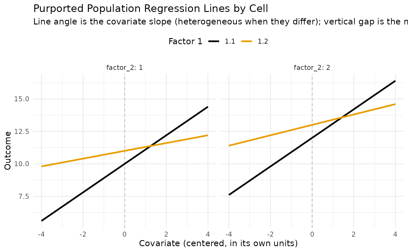
plot(dmar_composite_power_factorial_het): Draw the purported population values: the per-cell regression lines when population values were supplied, or the effect size lollipop otherwise.

Unequal Residual Variances When the Cell Correlations Differ

In cell c the residual variance is \(\tau_c^2 = \sigma^2 (1 - \rho_c^2)\), so cell correlations that differ in absolute value leave the cells with different residual variances. Averaging the squared correlations, which is what \(\sigma^2(1 - \bar{\rho^2})\) does, gets the expected pooled error right and its distribution wrong: the residual sum of squares is \(\sum_c \tau_c^2 Q_c\) with the \(Q_c\) independent chi square variables, a mixture of scaled chi squares with the same mean and a larger spread than the single scaled chi square the shared-error integral integrates over. The numerators are affected too. The covariate effect is the average cell slope and a slope effect is a contrast among the cell slopes, and cell slopes estimated with different residual variances give estimators of those two that are correlated, so the tests are not independent even given the error estimate.

Every power the function reports is then an approximation, and the output says so. composite_power is reported as approximate_composite_power, each power_<label> as approximate_power_<label>, and a planned sample size as approximate_n_per_cell and approximate_N, because that size is the smallest one at which the approximation reaches desired_power rather than a size known to attain it. The numbers do not change; the names do, and only in this case. Equal absolute cell correlations, including cells whose correlations share a magnitude and differ in sign, are the exact case and keep the ordinary names.

The error has no guaranteed sign, and it grows with the spread of the cell correlations rather than shrinking with N. Treat the number as an approximation and confirm a design you intend to run by simulating it: draw each cell's errors with its own residual standard deviation \(\sigma \sqrt{1 - \rho_c^2}\), fit the same model, and count the replications in which every effect in the composite is significant. The two-group help page reports the size of the departure over a range of correlation gaps.

The effect size interface is a special case worth naming. Supplying f or partial_eta_squared for each effect states the effects directly and says nothing about the cell correlations, so the function has nothing to detect unequal residual variances from and labels the table exact. If the design those effect sizes came from has cell correlations that differ in absolute value, the same approximation applies and the labels will not tell you; supply correlations instead when you want the function to keep track of it.

The figure

When the population values are supplied, plot() draws the population regression line in each cell over the covariate, so heterogeneous slopes show as lines of different angle and mean effects as vertical separation, colored by the first factor and faceted by any others. When effect sizes are supplied instead, it draws the effect size lollipop of ss_power_composite_factorial_ancova. Either way the composite power is in the subtitle. Requires ggplot2.

References

Maxwell, S. E., Delaney, H. D., & Kelley, K. (2027). Designing experiments and analyzing data: A model comparison perspective (4th ed.). Routledge. (See Chapter 9 on the analysis of covariance and heterogeneity of regression, and Chapter 7 on factorial designs.)

Author

Ken Kelley kkelley@nd.edu

Examples

# A 2 by 2 design whose conclusion needs a main effect and evidence that the
# covariate slope differs across the first factor. Effect sizes stated
# directly: the main effect (mean), the average covariate effect, and the
# factor 1 by covariate slope heterogeneity.
ss_power_composite_factorial_ancova_het(
  factor_levels = c(2, 2),
  effects = list(list(type = "mean",      factors = 1,  f = 0.25),
                 list(type = "covariate",               f = 0.40),
                 list(type = "slope",      factors = 1,  f = 0.20)),
  desired_power = 0.80)
#>  term                      value
#>  necessary_n_per_cell      55   
#>  necessary_N               220  
#>  composite_power           0.805
#>  residual_df               212  
#>  power_1                   0.958
#>  power_covariate           1    
#>  power_cov_x_1             0.84 
#>  f_1                       0.25 
#>  f_covariate               0.4  
#>  f_cov_x_1                 0.2  
#>  df_1                      1    
#>  df_covariate              1    
#>  df_cov_x_1                1    
#>  noncentral_parm_1         13.8 
#>  noncentral_parm_covariate 35.2 
#>  noncentral_parm_cov_x_1   8.8  
#>  cells                     4    
#>  alpha_level               0.05 
#>  desired_power             0.8  

# The same design from population values: cell means, a covariate-outcome
# correlation per cell (they differ across factor 1, so the slopes do), and a
# common within-cell SD. plot() then draws the per-cell regression lines.
cell_means <- matrix(c(10, 12,
                       11, 13), nrow = 2, byrow = TRUE)
cell_rho   <- matrix(c(0.55, 0.55,
                       0.15, 0.20), nrow = 2, byrow = TRUE)
fit <- ss_power_composite_factorial_ancova_het(
  factor_levels = c(2, 2), means = cell_means, correlations = cell_rho,
  sigma = 4, sd_cov = 2,
  effects = list(list(type = "mean",      factors = 1),
                 list(type = "covariate"),
                 list(type = "slope",      factors = 1)),
  n_per_cell = 40)
#> Warning: The cell correlations differ in absolute value, so the cells' residual variances differ and the shared-error composite power is an approximation whose error grows with the spread of the correlations. The powers are reported as approximate_* rows, and a planned sample size as approximate_n_per_cell, because neither is exact; confirm a final design by simulation.
fit
#>  term                        value
#>  specified_n_per_cell        40   
#>  specified_N                 160  
#>  approximate_composite_power 0.299
#>  residual_df                 152  
#>  approximate_power_1         0.406
#>  approximate_power_covariate 0.999
#>  approximate_power_cov_x_1   0.733
#>  f_1                         0.137
#>  f_covariate                 0.397
#>  f_cov_x_1                   0.205
#>  df_1                        1    
#>  df_covariate                1    
#>  df_cov_x_1                  1    
#>  noncentral_parm_1           3    
#>  noncentral_parm_covariate   25.2 
#>  noncentral_parm_cov_x_1     6.75 
#>  cells                       4    
#>  alpha_level                 0.05 
plot(fit)


# The one-factor, two-level case is the two-group composite ANCOVA.
ss_power_composite_factorial_ancova_het(
  factor_levels = 2,
  means = c(-0.25, 0.25), correlations = c(0.1, 0.5), sigma = 1,
  effects = list(list(type = "mean", factors = 1),
                 list(type = "slope", factors = 1)),
  n_per_cell = 100)
#> Warning: The cell correlations differ in absolute value, so the cells' residual variances differ and the shared-error composite power is an approximation whose error grows with the spread of the correlations. The powers are reported as approximate_* rows, and a planned sample size as approximate_n_per_cell, because neither is exact; confirm a final design by simulation.
#>  term                        value
#>  specified_n_per_cell        100  
#>  specified_N                 200  
#>  approximate_composite_power 0.825
#>  residual_df                 196  
#>  approximate_power_1         0.965
#>  approximate_power_cov_x_1   0.855
#>  f_1                         0.268
#>  f_cov_x_1                   0.214
#>  df_1                        1    
#>  df_cov_x_1                  1    
#>  noncentral_parm_1           14.4 
#>  noncentral_parm_cov_x_1     9.2  
#>  cells                       2    
#>  alpha_level                 0.05