Simulate Data From a Logistic Change (Growth) Model

Generates longitudinal data from a random-coefficients logistic change model: each unit (a person, an animal, a tree) follows an S-shaped (sigmoidal) curve with a lower and an upper asymptote and a symmetric point of inflection, the parameters vary randomly across units, and each measurement adds level-one error. The deterministic part of the four parameter logistic curve is $$\mu(t) = \frac{\alpha}{1 + \exp(-\gamma (t - \beta))} + \zeta,$$ the parameterization of Kelley (2005, 2008), which generalizes the three parameter logistic of the literature (Ratkowsky, 1983) by adding $\zeta$ so the lower asymptote is itself a modeled quantity rather than fixed at zero.

Usage

simulate_longitudinal_logistic(
  n,
  target_times = NULL,
  fixed_parameters,
  time_range = NULL,
  occasions = NULL,
  time_distribution = "uniform",
  random_variances = 0,
  random_correlation = NULL,
  error_variance = NULL,
  reliability = NULL,
  error_structure = c("independent", "ar1", "compound_symmetry", "toeplitz"),
  error_correlation = NULL,
  timing_sd = 0
)

Arguments

n

A single positive integer, the number of units (persons, animals, trees, classrooms) whose trajectories are drawn, or a vector giving the number of units for each population, one entry per parameter vector in fixed_parameters.

target_times

Numeric vector of the nominal measurement times, one shared schedule for every unit. Give either this or time_range.

fixed_parameters

The population parameters c(alpha = , beta = , gamma = , zeta = ) (an unnamed length-4 vector is taken in that order), or a list of such vectors, one per population (distinct data generating parameter vectors):

alpha: The total change: the curve travels alpha units from the lower asymptote zeta to the upper asymptote $\alpha + \zeta$ (for $\gamma > 0$).
beta: The point of inflection on the time axis: the moment of fastest change, at which exactly half the total change has occurred (the curve passes through $\alpha/2 + \zeta$). The inflection of the logistic is symmetric: the approach to the ceiling mirrors the departure from the floor.
gamma: The curvature: how sharply the curve rises through its inflection. Negative values flip the curve to decreasing.
zeta: The lower asymptote (for $\gamma > 0$), freeing the curve's floor from the fixed zero of the three parameter logistic. The intercept is $\phi = \alpha / (1 + \exp(\gamma \beta)) + \zeta$.

time_range

Alternative to target_times: c(lower, upper) bounds from which each unit draws its own measurement times, so no two units share a schedule (e.g., age in weeks at testing rather than a fixed grade). Requires occasions; with time_range, the level-one error must be a single error_variance with the default independent structure, and timing_sd does not apply.

occasions

With time_range: a single positive integer (every unit measured the same number of times) or c(min, max), from which each unit's number of measurement times is drawn uniformly.

time_distribution

Distribution of the unit-specific times over time_range; currently "uniform".

random_variances

Between-unit variances of (alpha, beta, gamma, zeta), a single number recycled to all four or a length-4 vector. Default 0. A named vector over any subset of the parameter names (e.g., c(beta = 1.2)) varies only those named and leaves the rest fixed.

random_correlation

Optional 4-by-4 correlation matrix among the random parameters; default uncorrelated.

error_variance, reliability, error_structure, error_correlation, timing_sd

The level-one error and assessment-time machinery, with the same meaning as in simulate_longitudinal_polynomial: specify exactly one of error_variance or reliability (solved here through the first-order delta method true-score variance; because the curve is nonlinear in its parameters, that approximation, and the reliability_by_occasion attribute with it, can drift from the realized variance ratio when the random variances are large relative to the mean curve); error_structure and error_correlation set the across-occasion error correlation; timing_sd jitters the actual assessment times.

Value

A long-format data.frame with columns id, population, occasion, target_time, time, true_score, and y, directly usable with plot_trajectories and nonlinear mixed-model fitters such as nlme::nlme(). Attributes carry the model, fixed_parameters, random_covariance, error_variance, error_covariance, reliability_by_occasion, and schedule ("shared" or "unit_specific").

Details

Every parameter is a landmark of the change process: the floor (zeta), the ceiling ($\alpha + \zeta$), when change is fastest (beta), and how concentrated the change is around that moment (gamma). The logistic is the $\delta = 1$ special case of the Richards curve (simulate_longitudinal_richards); its inflection always sits at 50% of the total change, which is the substantive assumption a researcher accepts in choosing it (Kelley, 2005, 2008).

References

Kelley, K. (2005). Estimating nonlinear change models in heterogeneous populations when class membership is unknown: Defining and developing the latent classification differential change model (Doctoral dissertation). University of Notre Dame.

Kelley, K. (2008). Nonlinear change models in populations with unobserved heterogeneity. Methodology, 4(3), 97–112.

Ratkowsky, D. A. (1983). Nonlinear regression modeling: A unified practical approach. Marcel Dekker.

Author

Ken Kelley kkelley@nd.edu

Examples

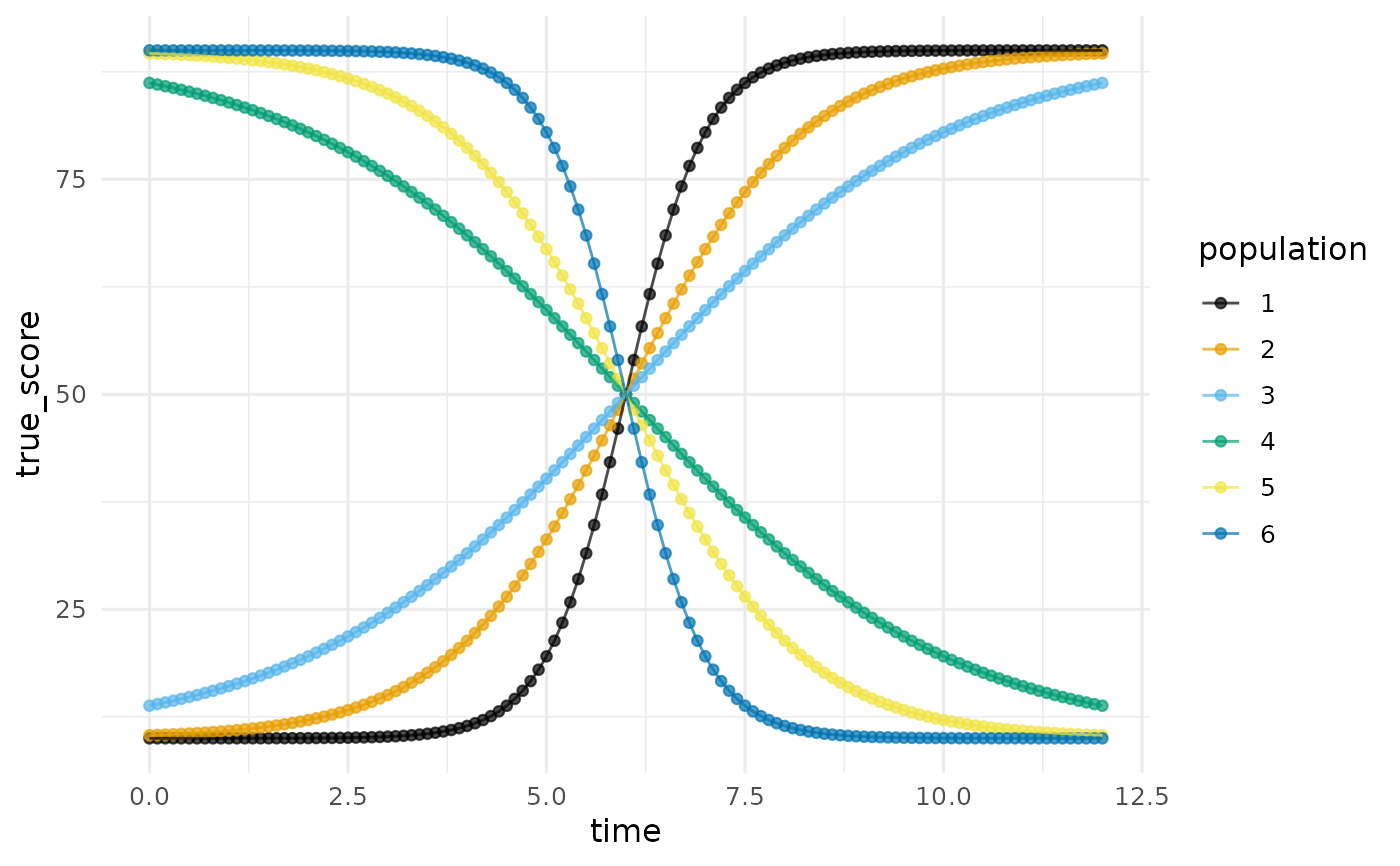
# A six-curve panel in the style of the growth-curve illustrations
# in Kelley (2005): floor 10 and ceiling 90 throughout, so every
# curve crosses its inflection at the same height (50, half the
# total change). The rising curves share beta = 6 and differ only in
# curvature; the falling curves mirror them. Each curve is its own population
# of size one, so a single call draws the whole panel.
panel <- simulate_longitudinal_logistic(
  n = 1, target_times = seq(0, 12, by = 0.1),
  fixed_parameters = list(
    c(alpha = 80, beta = 6, gamma =  2.0, zeta = 10),
    c(alpha = 80, beta = 6, gamma =  0.9, zeta = 10),
    c(alpha = 80, beta = 6, gamma =  0.5, zeta = 10),
    c(alpha = 80, beta = 6, gamma = -0.5, zeta = 10),
    c(alpha = 80, beta = 6, gamma = -0.9, zeta = 10),
    c(alpha = 80, beta = 6, gamma = -2.0, zeta = 10)),
  error_variance = 0
)
plot_trajectories(panel, id = "id", time = "time",
                  outcome = "true_score", group = "population")


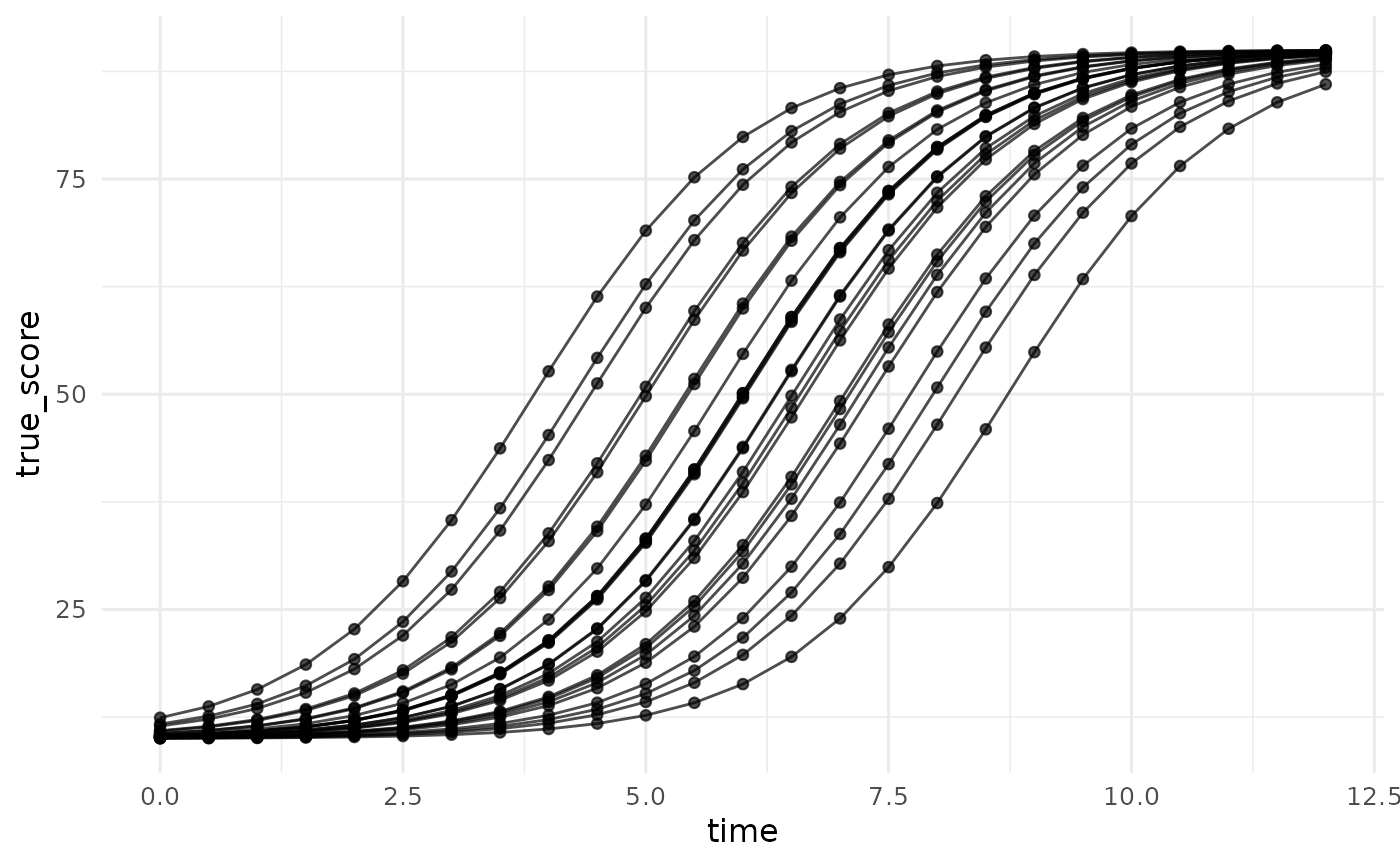
# Individual differences in a single parameter: only the inflection
# time varies (a named entry leaves the other variances at zero), so
# every learner shares the floor and the ceiling but hits fastest
# growth on a different week.
set.seed(113)
d_beta <- simulate_longitudinal_logistic(
  n = 25, target_times = seq(0, 12, by = 0.5),
  fixed_parameters = c(alpha = 80, beta = 6, gamma = 0.9, zeta = 10),
  random_variances = c(beta = 1.2), error_variance = 0
)
plot_trajectories(d_beta, id = "id", time = "time",
                  outcome = "true_score")


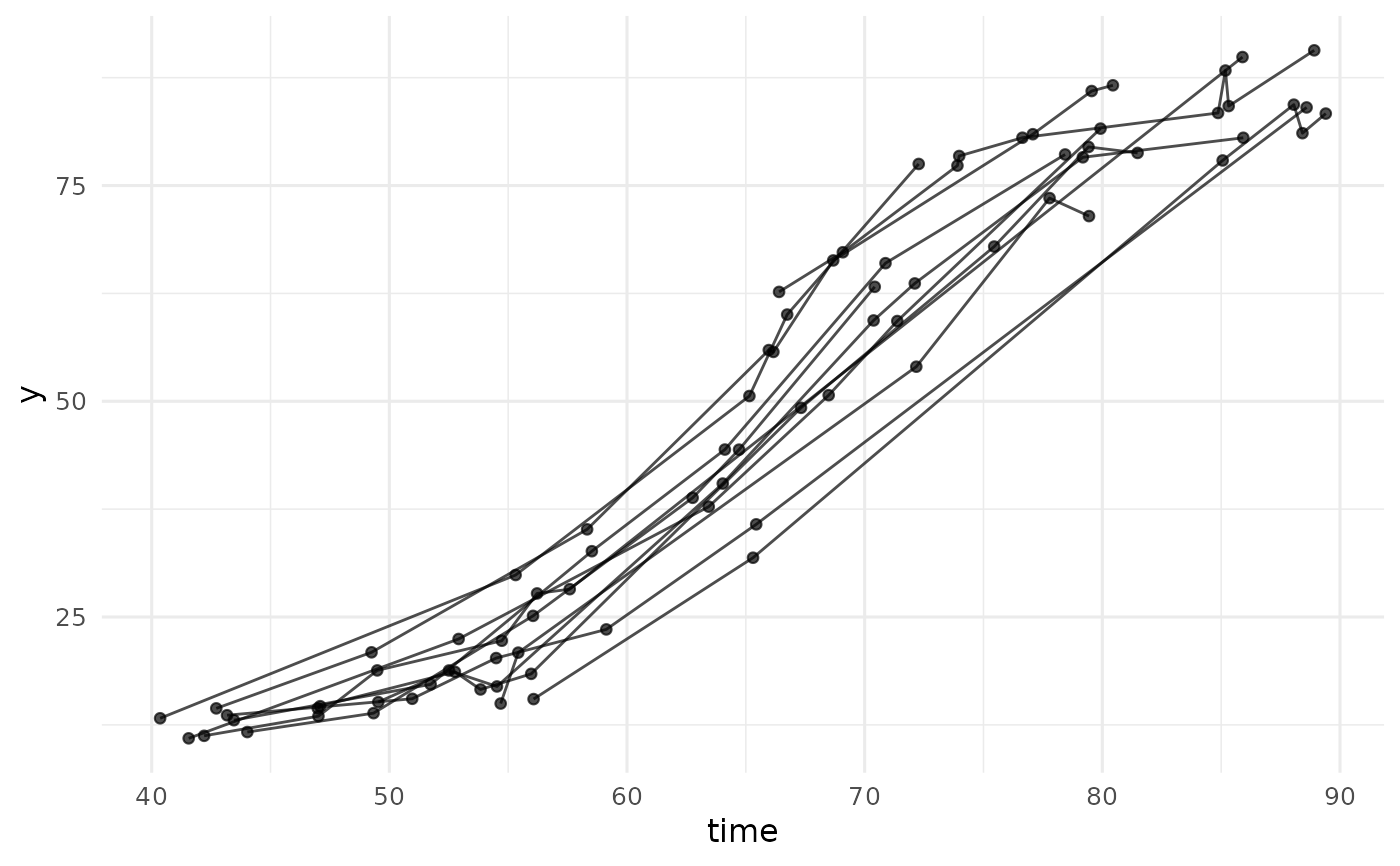
# Unit-specific measurement times: each child is tested at their own
# ages, drawn uniformly between 40 and 90 weeks with five to nine
# visits each, rather than on one shared schedule.
set.seed(113)
d_ages <- simulate_longitudinal_logistic(
  n = 12, time_range = c(40, 90), occasions = c(5, 9),
  fixed_parameters = c(alpha = 80, beta = 65, gamma = 0.15, zeta = 10),
  random_variances = c(beta = 16), error_variance = 4
)
plot_trajectories(d_ages, id = "id", time = "time", outcome = "y")


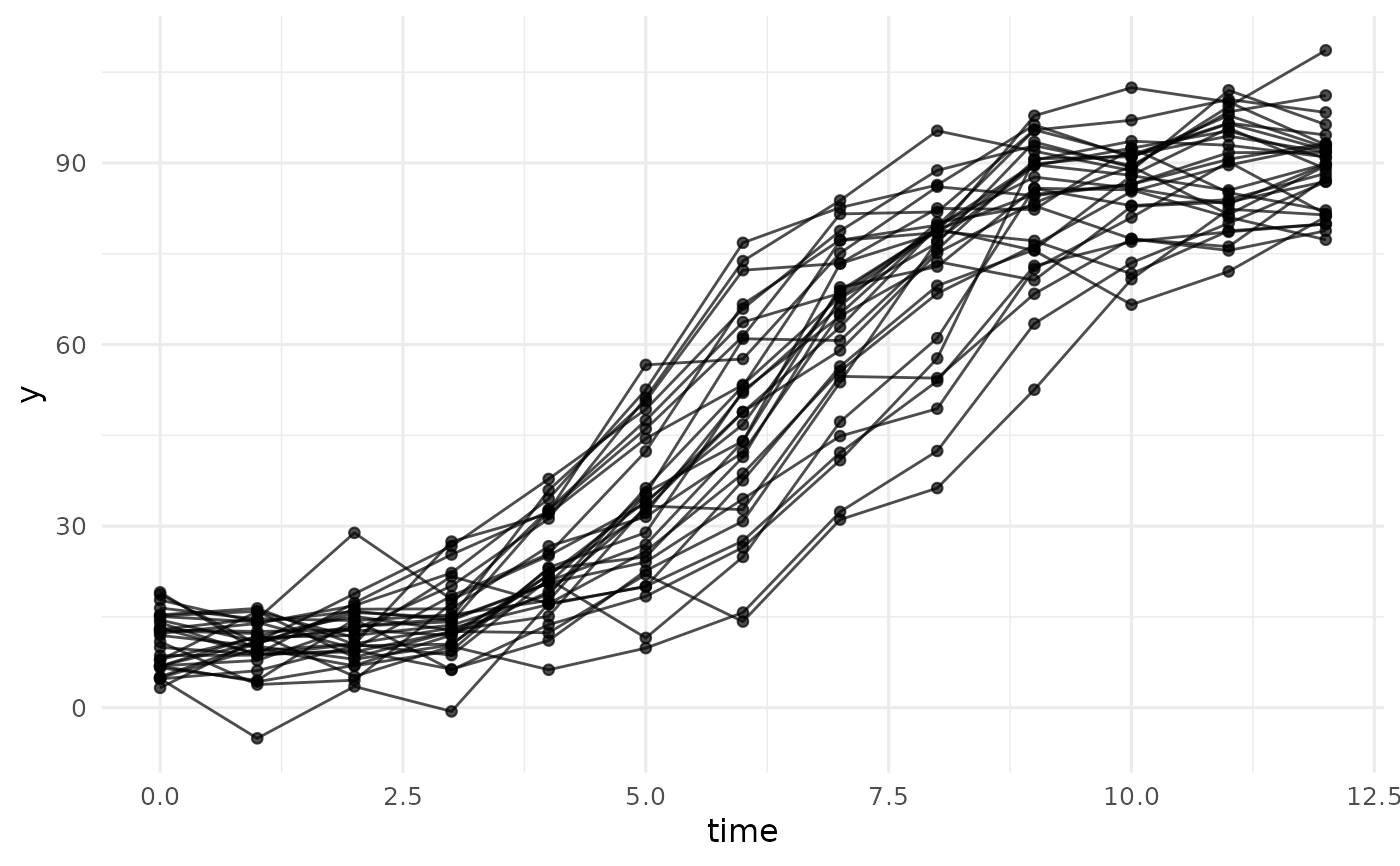
# Individual differences in every parameter, plus level-one error:
# skill acquisition from a floor near 10 to a ceiling near 90,
# fastest around week 6.
set.seed(113)
d <- simulate_longitudinal_logistic(
  n = 30, target_times = 0:12,
  fixed_parameters = c(alpha = 80, beta = 6, gamma = 0.9, zeta = 10),
  random_variances = c(alpha = 36, beta = 1, gamma = 0.01, zeta = 9),
  error_variance = 16
)
plot_trajectories(d, id = "id", time = "time", outcome = "y")