The Teacher Expectancy Meta-Analysis: Reproducing Raudenbush (1984)

In 1968, Pygmalion in the Classroom (Rosenthal & Jacobson) reported that telling teachers certain randomly chosen children were about to bloom intellectually raised those children’s IQ. The single study (shipped in DMAR as pygmalion, and the running analysis of covariance example in Maxwell, Delaney, and Kelley’s Designing Experiments and Analyzing Data) set off fourteen years of replications with wildly varying results. Raudenbush (1984) synthesized 18 of those experiments and asked the question that resolved the controversy: not whether there is an expectancy effect, but why the studies disagree. His answer: the longer teachers had known their pupils before the expectancy induction, the smaller the effect. Credible deception is the Achilles’ heel of the design.

This vignette reproduces the paper’s analyses with DMAR’s synthesis functions, then reanalyzes the data with modern random effects machinery. The single Pygmalion study and this literature are deliberately kept as separate data sets: one is a famous experiment, the other is the evidence about the claim.

The Data

The 1984 Table 1, at the condition level (Pellegrini & Hicks ran a tester-aware and a tester-blind condition):

data(teacher_expectancy)
teacher_expectancy[, c("author", "weeks", "tester", "d", "p_one_tailed")]
#>                                author weeks tester     d p_one_tailed
#> 1           Rosenthal, Baratz, & Hall     2  aware  0.02        0.401
#> 2  Conn, Edwards, Rosenthal, & Crowne    21  aware  0.14        0.206
#> 3                         Jose & Cody    19  aware -0.03        0.791
#> 4   Pellegrini & Hicks (tester aware)     0  aware  0.85        0.003
#> 5   Pellegrini & Hicks (tester blind)     0  blind  0.19        0.242
#> 6                   Evans & Rosenthal     3  aware -0.04        0.709
#> 7            Fielder, Cohen, & Feeney    17  blind -0.02        0.595
#> 8                  Fleming & Anttonen     2  blind  0.05        0.224
#> 9                            Claiborn    24  aware -0.13        0.928
#> 10                             Kester     0  aware  0.27        0.050
#> 11                            Maxwell     1  blind  0.55        0.002
#> 12                             Carter     0  blind  0.30        0.043
#> 13                            Flowers     0  blind  0.18        0.210
#> 14                            Keshock     1  blind -0.01        0.528
#> 15                          Henrikson     2  blind  0.16        0.250
#> 16                               Fine    17  aware -0.13        0.877
#> 17                           Ginsburg     7  aware -0.02        0.519
#> 18                            Grieger     5  blind -0.06        0.637
#> 19               Rosenthal & Jacobson     1  aware  0.21        0.016

For the analyses with the 18 studies as units, Raudenbush merged the two Pellegrini and Hicks conditions into their study-level values (d = 0.52, one-tailed p = .010; see ?teacher_expectancy):

s   <- teacher_expectancy[-c(4, 5), ]
d18 <- append(s$d,             0.52, after = 3)
p18 <- append(s$p_one_tailed,  .010, after = 3)
wk18 <- append(s$weeks,           0, after = 3)
ne18 <- append(s$n_experimental, 22, after = 3)
nc18 <- append(s$n_control,      22, after = 3)
round(c(mean = mean(d18), sd = sd(d18), max = max(d18), min = min(d18)), 2)
#>  mean    sd   max   min 
#>  0.11  0.20  0.55 -0.13

These match the paper’s summary exactly (M = 0.11, SD = 0.20, range 0.55 to -0.13).

Are the Studies Significant in Combination? (Table 2)

Raudenbush opened with four classical combined significance tests, which combine_p() provides in one call. The weights for the Mosteller-Bush weighted method are the studies’ degrees of freedom:

df18 <- ne18 + nc18 - 2
combine_p(p18, weights = df18)

term	value
fisher_chi_square	62.2
fisher_df	36
fisher_p	0.0043
edgington_sum_p	7
edgington_p	0.0509
stouffer_z	2.2
stouffer_p	0.0139
stouffer_weighted_z	0.87
stouffer_weighted_p	0.1922
k	18

Raudenbush’s Table 2 reports three of the four rejecting the null: Fisher’s chi square(36) = 62.17, Edgington’s sum of 6.84 (p = .04), and the adding-Zs test (his z = 2.12, p = .017), with only the df-weighted variant not rejecting. Recomputed here from the tabled one-tailed p-values, Fisher (chi square(36) = 62.17, p = .0043) and adding-Zs (z = 2.20, p = .0139) reject as he found, but Edgington’s sum comes to 6.996 rather than 6.84 and its p-value lands at .0509, a hair past the line his rounding placed it inside. A method whose decision flips with the third decimal of the inputs is telling you the evidence is borderline, not settled; the two sturdy rejections and the df-weighted non-rejection (z = 0.87, p = .19) carry the real message. That disagreement is the first finding: the larger studies found smaller effects, so something about the studies, not just sampling error, drives the variation.

Why Do the Studies Disagree? The Prior-Contact Contrast

The paper’s central hypothesis: the more weeks teachers had known their pupils before the induction, the less credible the deception, the smaller the effect.

plot(d18 ~ wk18,
     xlab = "Weeks of teacher-student contact before induction",
     ylab = "Effect size d", pch = 16)

The raw correlation and Raudenbush’s linearized (reciprocal-transformed) version:

round(c(r = cor(d18, wk18),
        r_transformed = cor(-1 / (1 + d18), -1 / (2 + wk18))), 2)
#>             r r_transformed 
#>         -0.55         -0.76

(The paper reports -.55 and -.77.) The formal test is a Rosenthal-Rubin contrast among the effect sizes, with weights inversely proportional to weeks of prior contact and the standard large-sample variance for each d:

v18 <- (ne18 + nc18) / (ne18 * nc18) + d18^2 / (2 * (ne18 + nc18))
meta_contrast(d18, v18, weights = 1 / (wk18 + 2))
#> Contrast weights mean-centered to sum to zero.

term	value
estimate	0.432
se	0.156
z	2.76
p_value	0.0057
k	18

The z of about 2.75 (one-tailed p = .003 in the paper) supports the hypothesis. Raudenbush partitioned the total heterogeneity the way an ANOVA partitions sums of squares: the fixed effect fit gives Cochran’s Q,

fe <- meta_es(d18, v18, method = "fe")
fe[fe$term %in% c("Q", "Q_df", "Q_p"), ]

term	value
Q	14.9
Q_df	17
Q_p	0.5997

Confidence level: 95%

and the squared contrast statistic over Q is the proportion of heterogeneity the moderator explains (Raudenbush’s 52 percent; the package returns 0.51 from these inputs):

z_contrast <- meta_contrast(d18, v18, weights = 1 / (wk18 + 2))$value[3]
#> Contrast weights mean-centered to sum to zero.
round(z_contrast^2 / fe$value[fe$term == "Q"], 2)
#> [1] 0.51

Note the instructive subtlety: the omnibus Q (14.9 on 17 df) would not itself reject homogeneity. A diffuse test looked at the same data and saw nothing; the focused contrast, specified in advance from a substantive hypothesis, saw the structure. That lesson, prefer focused model comparisons to omnibus tests, is the same one Maxwell, Delaney, and Kelley (2027) teach for single studies.

Low- Versus High-Contact Studies (Table 3)

Dichotomizing at two weeks of prior contact:

lo <- wk18 <= 2
round(c(mean_low = mean(d18[lo]), mean_high = mean(d18[!lo])), 2)
#>  mean_low mean_high 
#>      0.22     -0.04
combine_p(p18[lo],  weights = df18[lo])    # 10 low-contact studies

term	value
fisher_chi_square	54.2
fisher_df	20
fisher_p	< 0.0001
edgington_sum_p	1.73
edgington_p	0.0002
stouffer_z	4.15
stouffer_p	< 0.0001
stouffer_weighted_z	2.52
stouffer_weighted_p	0.0059
k	10

combine_p(p18[!lo], weights = df18[!lo])   # 8 high-contact studies

term	value
fisher_chi_square	7.98
fisher_df	16
fisher_p	0.9494
edgington_sum_p	5.26
edgington_p	0.9389
stouffer_z	-1.34
stouffer_p	0.9104
stouffer_weighted_z	-0.786
stouffer_weighted_p	0.7842
k	8

Every method finds the low-contact studies jointly significant (the paper: adding-Zs z = 4.16, weighted 2.52); none finds anything in the high-contact studies. Expectancy effects appear when, and only when, the teachers barely knew the children.

Tester Awareness (the Condition-Level Rows)

Could the effect be tester bias? Here the two Pellegrini and Hicks conditions matter, so the analysis runs at the condition level with an aware-versus-blind contrast:

d  <- teacher_expectancy$d
ne <- teacher_expectancy$n_experimental
nc <- teacher_expectancy$n_control
vi <- (ne + nc) / (ne * nc) + d^2 / (2 * (ne + nc))
aware <- teacher_expectancy$tester == "aware"
meta_contrast(d, vi, weights = ifelse(aware, 1 / sum(aware),
                                      -1 / sum(!aware)))

term	value
estimate	-0.0349
se	0.103
z	-0.338
p_value	0.7351
k	19

No main effect of tester awareness (the paper reports z = -0.36), and the low-contact effect held in both the aware and blind subsets: the prior-contact moderator is not an artifact of who administered the test.

A Modern Reanalysis

Raudenbush worked with the tools of 1984. The same questions today get a random effects model with REML, the Hartung-Knapp adjustment, a Q-profile interval for the between-study variance, and a prediction interval, all of which meta_smd() reports in one table (Hedges’ small-sample correction is on by default; the historical analyses above pooled raw d values):

meta_smd(smd = teacher_expectancy$d,
         n_1 = teacher_expectancy$n_experimental,
         n_2 = teacher_expectancy$n_control)

term	value
estimate	0.0544
se	0.0352
t	1.55
p_value	0.1392
lower_limit	-0.0195
upper_limit	0.128
prediction_lower	-0.0198
prediction_upper	0.129
tau2	0
tau2_lower	0
tau2_upper	0.048
tau	0
I2	0
I2_lower	0
I2_upper	64.6
H2	1
Q	16.7
Q_df	18
Q_p	0.5468
k	19

Confidence level: 95%

And the picture (the forest plot pools the raw d values, so its diamond sits fractionally left of the Hedges-corrected average in the table above):

plot_forest(d, vi, labels = teacher_expectancy$author,
            xlab = "Standardized mean difference (d)")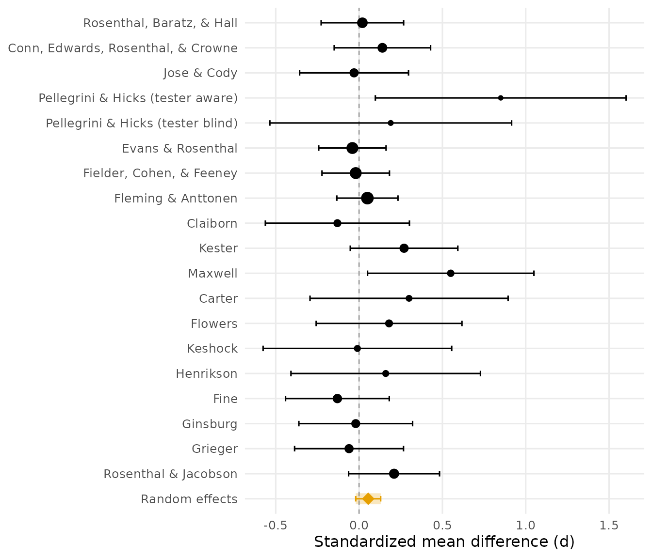

The pooled average is small and its confidence interval narrow, but the summary that respects the heterogeneity is conditional: pooling everything answers a question (“what is the average effect across these heterogeneous inductions?”) that the moderator analysis showed is the wrong one. Where will the next study land? It depends almost entirely on when the expectancy is induced.

References

Raudenbush, S. W. (1984). Magnitude of teacher expectancy effects on pupil IQ as a function of the credibility of expectancy induction: A synthesis of findings from 18 experiments. Journal of Educational Psychology, 76(1), 85–97.

Raudenbush, S. W., & Bryk, A. S. (1985). Empirical Bayes meta-analysis. Journal of Educational Statistics, 10(2), 75–98.

Rosenthal, R., & Jacobson, L. (1968). Pygmalion in the classroom. Holt, Rinehart & Winston.

Maxwell, S. E., Delaney, H. D., & Kelley, K. (2027). Designing experiments and analyzing data: A model comparison perspective (4th ed.). Routledge.

Ken Kelley