Composite Sample Size Planning for SEM: A Simple Model and a Latent Growth Curve

# Produced by tools/composite_sem_reference.R, which runs each of the eight
# calls in this vignette at G = 10000. Carried as literals because that sweep
# takes about an hour and cannot run while the document is being knitted.
ref <- list(
  med_at_100  = c(composite_power = 0.8692, power_a = 0.9883,
                  power_b = 0.9367, power_ab = 0.8692),
  med_plan    = c(necessary_N = 88, composite_power = 0.8052,
                  power_a = 0.9762, power_b = 0.9067, power_ab = 0.8052),
  med_plan_cp = c(necessary_N = 343, composite_power = 0.8143,
                  power_a = 1.0000, power_b = 1.0000, power_cp = 0.8143,
                  power_ab = 1.0000),
  med_aipe    = c(necessary_N = 238, composite_assurance = 0.3816,
                  mean_width_a = 0.2330, mean_width_b = 0.2499,
                  mean_width_ab = 0.1301),
  med_aipe_80 = c(necessary_N = 268, composite_assurance = 0.8082,
                  mean_width_a = 0.2196, mean_width_b = 0.2355,
                  mean_width_ab = 0.1224),
  lgm_at_150  = c(composite_power = 0.6700, power_mu_s = 1.0000,
                  power_cov_is = 0.6700),
  lgm_plan    = c(necessary_N = 201, composite_power = 0.8008,
                  power_mu_s = 1.0000, power_cov_is = 0.8008),
  lgm_aipe    = c(necessary_N = 220, composite_assurance = 0.8197,
                  width_within_desired_mu_s = 0.8197,
                  width_within_desired_cov_is = 0.9956)
)

The sample sizes these calls print are not planning values. Every call below uses G = 25 Monte Carlo replications so the document knits in about twenty seconds. At that many replications a reported proportion carries a simulation standard error near 0.10, and the necessary $N$ inherits it.

So that a reader can see both the method and the answer, every result is reported beside the same call at G = 10000, which is the column to read. The gap is not small: the first plan below needs $N = 88$ at 10,000 replications, and G = 25 misses it. Those reference values were produced by tools/composite_sem_reference.R, which runs the identical calls at G = 10000 and takes about an hour; the script is in the maintained repository and is not shipped with the package. A plan you intend to defend is worth G = 1000 or more, which is what every G argument in this document should become before its answer is used.

Most studies that fit a structural equation model state more than one hypothesis, and the paper’s conclusion holds only when all of them do. A study can have adequate statistical power for each hypothesis on its own and still be underpowered for the conjunction, because the probability that every test succeeds in the same study is smaller, often much smaller, than any single test’s power (Maxwell, 2004). The same logic applies to accuracy: a design is only as informative as its widest confidence interval of interest. Sample size planning should therefore be done for the set of parameters a study’s conclusion rests on, not for one parameter at a time.

DMAR implements this with two functions, both driven by a priori Monte Carlo simulation (Muthén & Muthén, 2002; Maxwell, Kelley, & Rausch, 2008):

ss_power_composite_sem() finds the smallest $N$ at which every parameter of interest is statistically significant in the same study with a desired probability (the composite power), or reports that probability at a given $N$ ;
ss_aipe_composite_sem() finds the smallest $N$ at which every confidence interval of interest is sufficiently narrow, in expectation or with a stated assurance for the joint event, the accuracy in parameter estimation (AIPE) goal.

This vignette works through the same workflow twice: first for a simple model with observed variables, then for a latent growth curve model, where the parameters of interest include a latent mean. Both functions require to be installed.

The Workflow

Every plan is built from two model statements.

A population model, written in lavaan syntax with every parameter fixed to the value the researcher posits (from theory, prior studies, or pilot data; these are population values, never sample estimates). cov_sem() turns it into the population covariance matrix, and, when the model has a mean structure, the population mean vector.
The analysis model, the free model that would be fit to the data, with a label on each parameter of interest. The labeled set is the composite. Labels can also name quantities defined with :=, such as an indirect effect.

For a candidate $N$ , the planner draws G samples of size $N$ from the population, fits the analysis model to each, and records each labeled parameter’s test and confidence interval. Because the estimates come from one fitted model per sample, their dependence is reflected exactly; nothing is assumed about how the tests relate. A search over $N$ , seeded by an analytic Wald approximation, then brackets and bisects to the smallest sample size meeting the goals.

A Simple Model: Mediation Among Observed Variables

Suppose a training program (x) is thought to improve job performance (y) by building self-efficacy (m): the classic mediation structure with paths $a$ (from x to m), $b$ (from m to y holding x constant), the direct path $c'$ , and the indirect effect $ab$ . The claims the paper will make are that training builds self-efficacy, that self-efficacy carries into performance, and that the indirect effect is nonzero. Those three claims name the set: $a$ , $b$ , and $ab$ .

The Population

The residual variances below are chosen so every variable has unit variance, so the paths read as standardized effects: $a = 0.4$ , $b = 0.35$ , $c' = 0.15$ , and therefore $ab = 0.14$ .

pop_med <- "
  x ~~ 1*x
  m ~ 0.4*x
  m ~~ 0.84*m
  y ~ 0.35*m + 0.15*x
  y ~~ 0.813*y
"
cov_sem(pop_med)$sigma_theta
#>      m    y    x
#> m 1.00 0.41 0.40
#> y 0.41 1.00 0.29
#> x 0.40 0.29 1.00

The Analysis Model and the Parameters of Interest

The analysis model is free; the labels name the parameters of interest, and ab := a*b defines the indirect effect (its standard error comes from the delta method, as in lavaan itself).

med_model <- "
  m ~ a*x
  y ~ b*m + cp*x
  ab := a*b
"

Composite Power at a Candidate Sample Size

Suppose $N = 100$ is under consideration. parameters selects the labeled set; G is the number of Monte Carlo replications, kept at 25 here so the document knits quickly, and the seed makes the result reproducible. As the note at the top says, a plan you intend to defend is worth G = 1000 or more.

med_at_100 <- ss_power_composite_sem(
  model = med_model, pop_model = pop_med,
  parameters = c("a", "b", "ab"),
  N = 100, G = 25, seed = 113)
med_at_100

term	value
specified_N	100
composite_power	0.84
composite_power_mc_se	0.0733
power_a	0.96
power_b	0.96
power_ab	0.84
population_a	0.4
population_b	0.35
population_ab	0.14
alpha_level	0.05
replications	25
converged_replications	25


compare(med_at_100, ref$med_at_100,
        c("composite_power", "power_a", "power_b", "power_ab"))
#>                 G = 25 G = 10000
#> composite_power   0.84    0.8692
#> power_a           0.96    0.9883
#> power_b           0.96    0.9367
#> power_ab          0.84    0.8692

The power_a, power_b, and power_ab rows are the marginal powers, each the proportion of the G replications in which that parameter was significant. The composite_power row is the proportion in which all three were significant in the same replication: here 0.84, at most the smallest marginal power, and estimated with a simulation standard error of about 0.073. Because the three tests share one fitted model they are dependent, so the composite need not equal the product of the marginals; the simulation gets the joint probability right without any independence assumption.

The Necessary Sample Size

Planning replaces N with desired_power:

med_plan <- ss_power_composite_sem(
  model = med_model, pop_model = pop_med,
  parameters = c("a", "b", "ab"),
  desired_power = 0.80, G = 25, seed = 113)
med_plan

term	value
necessary_N	76
composite_power	0.8
composite_power_mc_se	0.08
power_a	1
power_b	0.96
power_ab	0.8
population_a	0.4
population_b	0.35
population_ab	0.14
alpha_level	0.05
replications	25
converged_replications	25
desired_power	0.8


compare(med_plan, ref$med_plan,
        c("necessary_N", "composite_power", "power_a", "power_b", "power_ab"))
#>                 G = 25 G = 10000
#> necessary_N      76.00   88.0000
#> composite_power   0.80    0.8052
#> power_a           1.00    0.9762
#> power_b           0.96    0.9067
#> power_ab          0.80    0.8052

A sample of $N = 88$ is the smallest at which the estimated composite power reaches 0.80, reading the reference column. The result carries the same broom summary as the rest of the ss_power_* family:

generics::tidy(med_plan)
#>          term estimate power
#> 1 sample_size       76   0.8

The Weakest Parameter Governs the Design

The direct path $c' = 0.15$ was deliberately left out of the set above. Adding it shows why the choice of the set is a substantive decision, not a formality:

med_plan_cp <- ss_power_composite_sem(
  model = med_model, pop_model = pop_med,
  parameters = c("a", "b", "cp", "ab"),
  desired_power = 0.80, G = 25, seed = 113)
med_plan_cp

term	value
necessary_N	353
composite_power	0.84
composite_power_mc_se	0.0733
power_a	1
power_b	1
power_cp	0.84
power_ab	1
population_a	0.4
population_b	0.35
population_cp	0.15
population_ab	0.14
alpha_level	0.05
replications	25
converged_replications	25
desired_power	0.8


compare(med_plan_cp, ref$med_plan_cp,
        c("necessary_N", "composite_power", "power_cp"))
#>                 G = 25 G = 10000
#> necessary_N     353.00  343.0000
#> composite_power   0.84    0.8143
#> power_cp          0.84    0.8143

Requiring the small direct path to be significant as well moves the necessary sample size from $N = 88$ to $N = 343$ . The composite is bounded by its weakest member, so the set should contain exactly the parameters the paper’s conclusion requires, and each addition is a design commitment with a visible price.

Accuracy for the Set: AIPE

When the research questions concern magnitudes, the goal is a sufficiently narrow confidence interval for every parameter of interest. desired_width states the full width per parameter, as a named vector so a width can never silently attach to the wrong parameter; the indirect effect, on its smaller scale, is held to a narrower interval here.

med_aipe <- ss_aipe_composite_sem(
  model = med_model, pop_model = pop_med,
  parameters = c("a", "b", "ab"),
  desired_width = c(a = 0.25, b = 0.25, ab = 0.15),
  G = 25, seed = 113)
med_aipe

term	value
necessary_N	245
composite_assurance	0.52
mean_width_a	0.227
mean_width_b	0.249
mean_width_ab	0.125
width_within_desired_a	0.92
width_within_desired_b	0.56
width_within_desired_ab	0.96
desired_width_a	0.25
desired_width_b	0.25
desired_width_ab	0.15
population_a	0.4
population_b	0.35
population_ab	0.14
conf_level	0.95
replications	25
converged_replications	25

Confidence level: 95%


compare(med_aipe, ref$med_aipe,
        c("necessary_N", "composite_assurance", "mean_width_a",
          "mean_width_b", "mean_width_ab"))
#>                       G = 25 G = 10000
#> necessary_N         245.0000  238.0000
#> composite_assurance   0.5200    0.3816
#> mean_width_a          0.2271    0.2330
#> mean_width_b          0.2495    0.2499
#> mean_width_ab         0.1254    0.1301

With no assurance, the criterion is the expected width: the returned $N = 238$ is the smallest at which the mean simulated width of every interval is within its target. Widths vary from sample to sample, so a study of that size obtains all three sufficiently narrow intervals in only about 38 percent of its realizations (the composite_assurance row). Supplying an assurance plans against that joint event directly:

med_aipe_80 <- ss_aipe_composite_sem(
  model = med_model, pop_model = pop_med,
  parameters = c("a", "b", "ab"),
  desired_width = c(a = 0.25, b = 0.25, ab = 0.15),
  assurance = 0.80, G = 25, seed = 113)
med_aipe_80

term	value
necessary_N	262
composite_assurance	0.92
mean_width_a	0.222
mean_width_b	0.229
mean_width_ab	0.118
width_within_desired_a	1
width_within_desired_b	0.92
width_within_desired_ab	1
desired_width_a	0.25
desired_width_b	0.25
desired_width_ab	0.15
population_a	0.4
population_b	0.35
population_ab	0.14
conf_level	0.95
replications	25
converged_replications	25
assurance	0.8

Confidence level: 95%


compare(med_aipe_80, ref$med_aipe_80,
        c("necessary_N", "composite_assurance"))
#>                     G = 25 G = 10000
#> necessary_N         262.00  268.0000
#> composite_assurance   0.92    0.8082

A planning summary an author could report: with $N = 268$ , all three intervals are simultaneously no wider than their targets (0.25, 0.25, and 0.15) in an estimated 92 percent of studies, under the stated population model and a 95% confidence level.

A Latent Growth Curve

Now a longitudinal design: well-being measured at four annual waves, with individual change modeled by a linear latent growth curve. The intercept factor i is a person’s status at wave 1; the slope factor s is the person’s annual change. Two questions drive the study, and both must hold for the paper’s argument:

Is there average growth? The mean of the slope factor, $\mu_s$ .
Do people who start higher grow less? The intercept-slope covariance, $\sigma_{is}$ .

The first is a question about a latent mean, which is why the planners accept a population mean structure alongside the covariance structure.

The Population Growth Process

The posited population: average status 5 at wave 1, average growth 0.3 per year, intercept variance 1, slope variance 0.2, intercept-slope covariance $-0.15$ (a correlation of about $-0.34$ : those who start higher grow less), and residual variance 0.5 at every wave. Every parameter, including every intercept and latent mean, is fixed.

pop_lgm <- "
  i =~ 1*t1 + 1*t2 + 1*t3 + 1*t4
  s =~ 0*t1 + 1*t2 + 2*t3 + 3*t4
  i ~~ 1*i
  s ~~ 0.2*s
  i ~~ -0.15*s
  t1 ~~ 0.5*t1; t2 ~~ 0.5*t2; t3 ~~ 0.5*t3; t4 ~~ 0.5*t4
  t1 ~ 0*1; t2 ~ 0*1; t3 ~ 0*1; t4 ~ 0*1
  i ~ 5*1
  s ~ 0.3*1
"
lgm_pop <- cov_sem(pop_lgm)
lgm_pop$mu_theta
#>  t1  t2  t3  t4 
#> 5.0 5.3 5.6 5.9
lgm_pop$sigma_theta
#>      t1   t2   t3   t4
#> t1 1.50 0.85 0.70 0.55
#> t2 0.85 1.40 0.95 1.00
#> t3 0.70 0.95 1.70 1.45
#> t4 0.55 1.00 1.45 2.40

cov_sem() returns both moments the population implies: the wave means rise by 0.3 per year, and the wave variances and covariances follow from the growth factor variances, their covariance, and the residuals.

The population is worth seeing. Each light line below is one person’s model implied trajectory, drawn from the population distribution of $(i, s)$ ; the bold line is the average trajectory.

set.seed(113)
growth_factors <- MASS::mvrnorm(
  n = 40, mu = c(5, 0.3),
  Sigma = matrix(c(1, -0.15, -0.15, 0.2), 2, 2))
traj <- data.frame(
  person = rep(seq_len(40), each = 4),
  wave = rep(1:4, times = 40),
  wellbeing = growth_factors[rep(seq_len(40), each = 4), 1] +
    growth_factors[rep(seq_len(40), each = 4), 2] * rep(0:3, times = 40))

ggplot(traj, aes(wave, wellbeing, group = person)) +
  geom_line(color = "grey70", linewidth = 0.4) +
  geom_line(data = data.frame(person = 0, wave = 1:4,
                              wellbeing = 5 + 0.3 * 0:3),
            color = unname(grDevices::palette.colors(2)[2]),
            linewidth = 1.4) +
  labs(title = "The Population the Design Is Planned On",
       subtitle = "Individual latent trajectories; the bold line is the average trajectory",
       x = "Wave", y = "Well-being")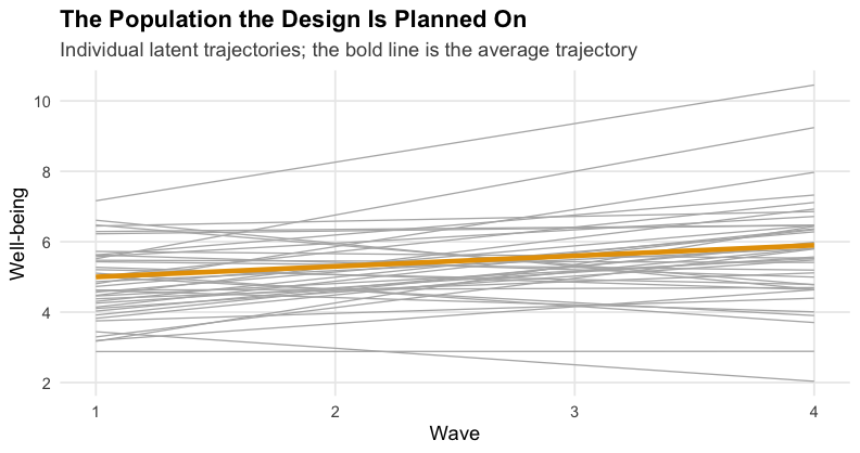

plot of chunk lgm-trajectories

The negative intercept-slope covariance is visible: trajectories that start high tend to tilt down relative to the average, so the fan narrows over time.

The Analysis Model

The analysis model is the same growth structure with its parameters free. Written for lavaan::sem(), the growth parameterization fixes the observed intercepts to zero and frees the latent means (this is exactly what lavaan::growth() does internally). The two parameters of interest carry labels.

lgm_model <- "
  i =~ 1*t1 + 1*t2 + 1*t3 + 1*t4
  s =~ 0*t1 + 1*t2 + 2*t3 + 3*t4
  i ~~ cov_is*s
  t1 ~ 0*1; t2 ~ 0*1; t3 ~ 0*1; t4 ~ 0*1
  i ~ 1
  s ~ mu_s*1
"

Composite Power for the Growth Questions

First, what does a candidate $N = 150$ deliver?

lgm_at_150 <- ss_power_composite_sem(
  model = lgm_model, pop_model = pop_lgm,
  parameters = c("mu_s", "cov_is"),
  N = 150, G = 25, seed = 113)
lgm_at_150

term	value
specified_N	150
composite_power	0.64
composite_power_mc_se	0.096
power_mu_s	1
power_cov_is	0.64
population_mu_s	0.3
population_cov_is	-0.15
alpha_level	0.05
replications	25
converged_replications	25


compare(lgm_at_150, ref$lgm_at_150,
        c("composite_power", "power_mu_s", "power_cov_is"))
#>                 G = 25 G = 10000
#> composite_power   0.64      0.67
#> power_mu_s        1.00      1.00
#> power_cov_is      0.64      0.67

The average growth of 0.3 per year is easy to detect (power_mu_s is 1), and the composite is governed almost entirely by the covariance question: power_cov_is is 0.64, and the composite power is 0.64. Planning for the pair:

lgm_plan <- ss_power_composite_sem(
  model = lgm_model, pop_model = pop_lgm,
  parameters = c("mu_s", "cov_is"),
  desired_power = 0.80, G = 25, seed = 113)
lgm_plan

term	value
necessary_N	216
composite_power	0.88
composite_power_mc_se	0.065
power_mu_s	1
power_cov_is	0.88
population_mu_s	0.3
population_cov_is	-0.15
alpha_level	0.05
replications	25
converged_replications	25
desired_power	0.8


compare(lgm_plan, ref$lgm_plan,
        c("necessary_N", "composite_power", "power_cov_is"))
#>                 G = 25 G = 10000
#> necessary_N     216.00  201.0000
#> composite_power   0.88    0.8008
#> power_cov_is      0.88    0.8008

About $N = 201$ participants are needed for both growth questions to be answered affirmatively in the same study with probability 0.80, under the stated population. A researcher who planned only for the slope mean, the headline effect, would have chosen a far smaller study and then usually failed to detect the covariance that the theory also requires.

Accuracy for the Growth Parameters

The magnitude of growth and of its dependence on initial status are usually the quantities of substantive interest, so the AIPE plan holds the slope mean to an interval no wider than 0.15 (that is, $\pm 0.075$ around an effect of 0.3 per year) and the covariance to 0.25, jointly, in 80 percent of studies:

lgm_aipe <- ss_aipe_composite_sem(
  model = lgm_model, pop_model = pop_lgm,
  parameters = c("mu_s", "cov_is"),
  desired_width = c(mu_s = 0.15, cov_is = 0.25),
  assurance = 0.80, G = 25, seed = 113)
lgm_aipe

term	value
necessary_N	220
composite_assurance	0.92
mean_width_mu_s	0.142
mean_width_cov_is	0.205
width_within_desired_mu_s	0.92
width_within_desired_cov_is	1
desired_width_mu_s	0.15
desired_width_cov_is	0.25
population_mu_s	0.3
population_cov_is	-0.15
conf_level	0.95
replications	25
converged_replications	25
assurance	0.8

Confidence level: 95%


compare(lgm_aipe, ref$lgm_aipe,
        c("necessary_N", "composite_assurance",
          "width_within_desired_mu_s", "width_within_desired_cov_is"))
#>                             G = 25 G = 10000
#> necessary_N                 220.00  220.0000
#> composite_assurance           0.92    0.8197
#> width_within_desired_mu_s     0.92    0.8197
#> width_within_desired_cov_is   1.00    0.9956

The accuracy goal needs $N = 220$ , and the width_within_desired_* rows show which target binds: the slope mean’s interval is the harder one to keep narrow at this $N$ . When both existence and magnitude matter, the defensible design uses the larger of the power and AIPE sample sizes, here $N = 220$ .

Practical Notes

Monte Carlo precision. Every power and proportion reported is an estimate from G replications with simulation standard error about $\sqrt{p(1-p)/G}$ , and the necessary $N$ inherits that uncertainty. The small G used here keeps the vignette quick; real plans deserve G = 1000 or more, and reporting the seed makes a plan reproducible.
Sensitivity to the population values. The plan is conditional on the posited population, exactly as in any sample size planning. Because the planner is itself a Monte Carlo study, sensitivity analysis is direct: rerun it with the alternative population values under consideration (a smaller slope mean, a weaker covariance) and compare the plans.
Convergence. Replications that fail to converge are redrawn and the summaries condition on convergence; frequent nonconvergence at small $N$ is itself design information, and the planners say so when it happens.
Variance parameters. Any labeled parameter can join the set, including a variance such as the slope variance. Its Wald test is reported like any other, but a variance near its boundary of zero is a case the two-sided Wald test treats roughly; interpret such a target with care.

References

Lai, K., & Kelley, K. (2011). Accuracy in parameter estimation for targeted effects in structural equation modeling: Sample size planning for narrow confidence intervals. Psychological Methods, 16(2), 127–148.

Maxwell, S. E. (2004). The persistence of underpowered studies in psychological research: Causes, consequences, and remedies. Psychological Methods, 9(2), 147–163.

Maxwell, S. E., Delaney, H. D., & Kelley, K. (2027). Designing experiments and analyzing data: A model comparison perspective (4th ed.). Routledge.

Maxwell, S. E., Kelley, K., & Rausch, J. R. (2008). Sample size planning for statistical power and accuracy in parameter estimation. Annual Review of Psychology, 59, 537–563.

Muthén, L. K., & Muthén, B. O. (2002). How to use a Monte Carlo study to decide on sample size and determine power. Structural Equation Modeling, 9(4), 599–620.

Rosseel, Y. (2012). lavaan: An R package for structural equation modeling. Journal of Statistical Software, 48(2), 1–36.

Ken Kelley

August 2026

The Workflow

A Simple Model: Mediation Among Observed Variables

The Population

The Analysis Model and the Parameters of Interest

Composite Power at a Candidate Sample Size

The Necessary Sample Size

The Weakest Parameter Governs the Design

Accuracy for the Set: AIPE

A Latent Growth Curve

The Population Growth Process

The Analysis Model

Composite Power for the Growth Questions

Accuracy for the Growth Parameters

Practical Notes

References